Climbing Hold Surface Roughness Analysis

Application Note | 3D Optical Profilometry

Climbing Hold Surface Roughness Analysis Using 3D Optical Profilometry

Measuring Texture, Porosity, and Topography on Bouldering Holds

Research & Experimental Testing

Walter Alabiso, PhD

Visual Design & Editorial

Andrew Shore

Introduction

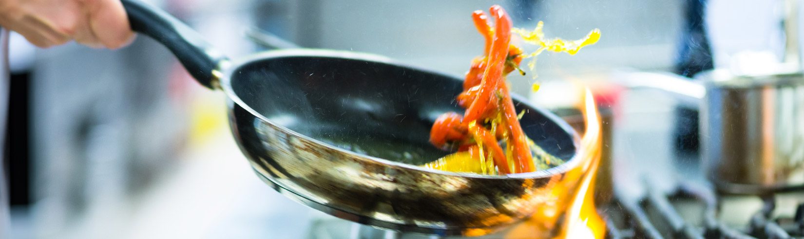
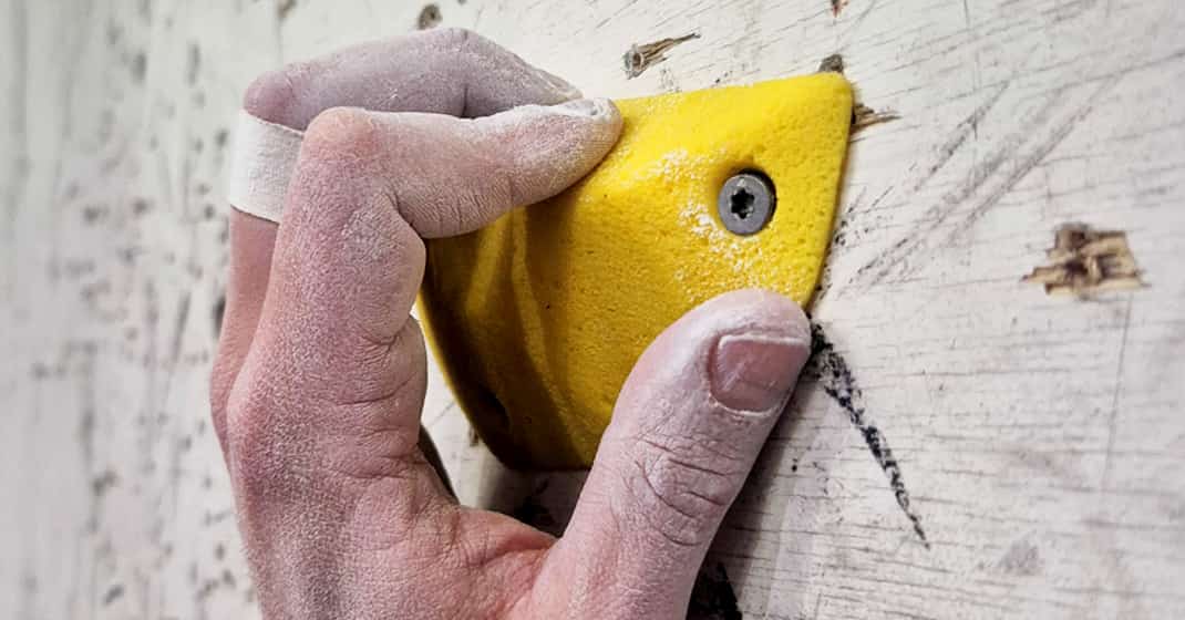
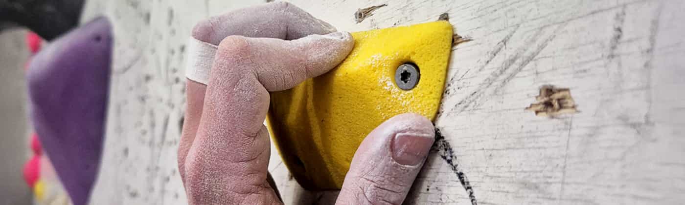
Bouldering is a demanding discipline that combines physical strength, precise body positioning, and an understanding of how the human body interacts with climbing surfaces. On slab routes, where the wall is angled below vertical and positive holds are limited or absent, a climber’s stability depends almost entirely on the tribological interaction between the body and the climbing hold surface.

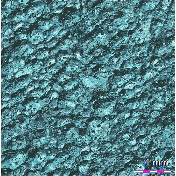
Climbing hold surface roughness plays a central role in this contact. Roughness provides the microtexture needed for smearing, a technique where high-friction rubber soles are pressed firmly against the surface to expand the effective contact area and generate adherence. A similar mechanism occurs at the fingers, where the ridges of fingerprints and the pliability of skin deform slightly against the hold’s surface features, creating grip through microscopic interlocking.

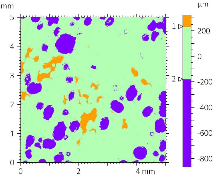
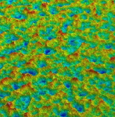
Porosity contributes to grip performance by absorbing moisture, sweat, or chalk at the contact interface, preventing the formation of a thin lubricating film that would reduce friction. Micro-cracks and surface flaws act as additional friction points, helping the climber maintain lateral tension against the hold surface. Because these features (roughness, porosity, and surface morphology) operate at different scales and interact differently depending on the hold, quantitative 3D surface measurement is essential for comparing how different climbing hold textures perform under real contact conditions.

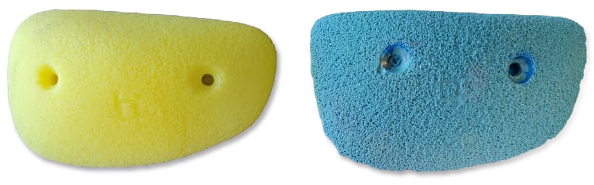
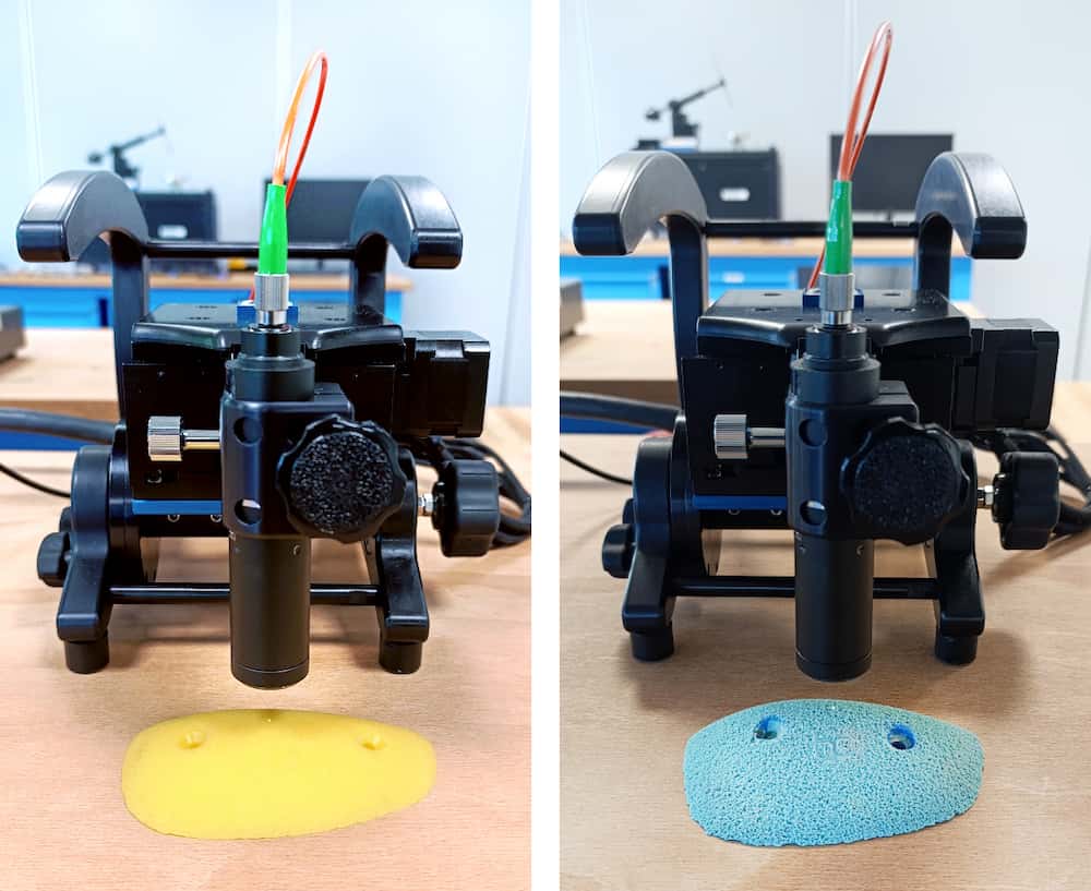
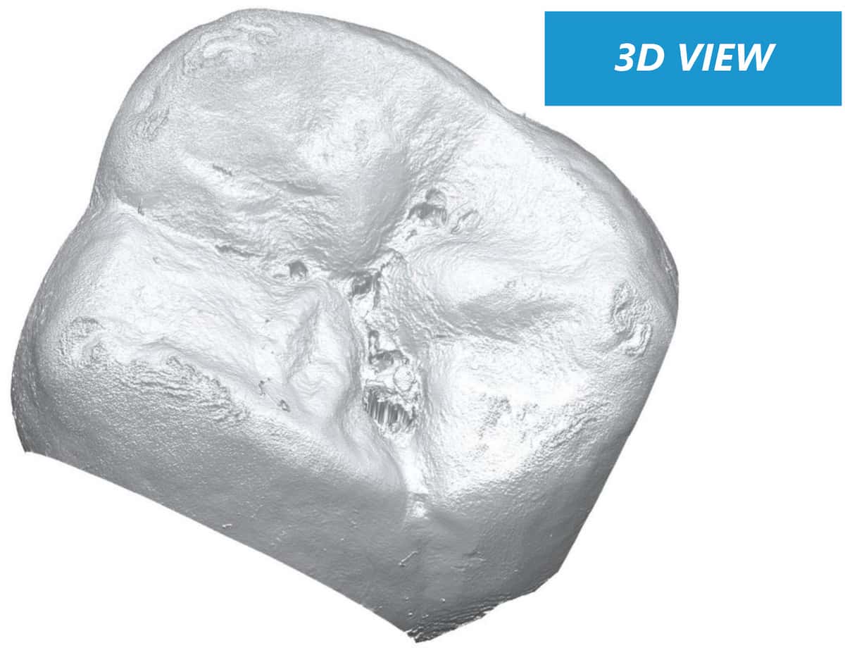
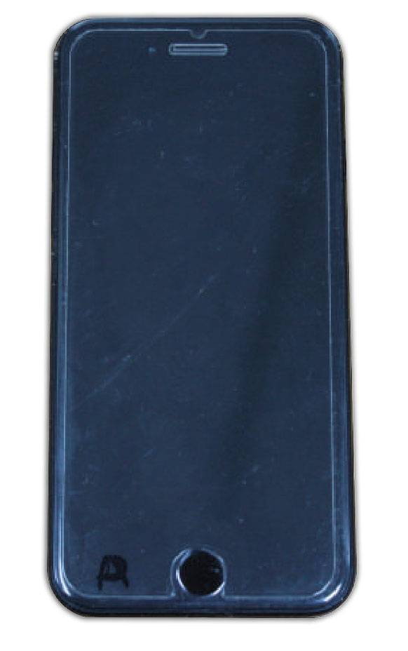
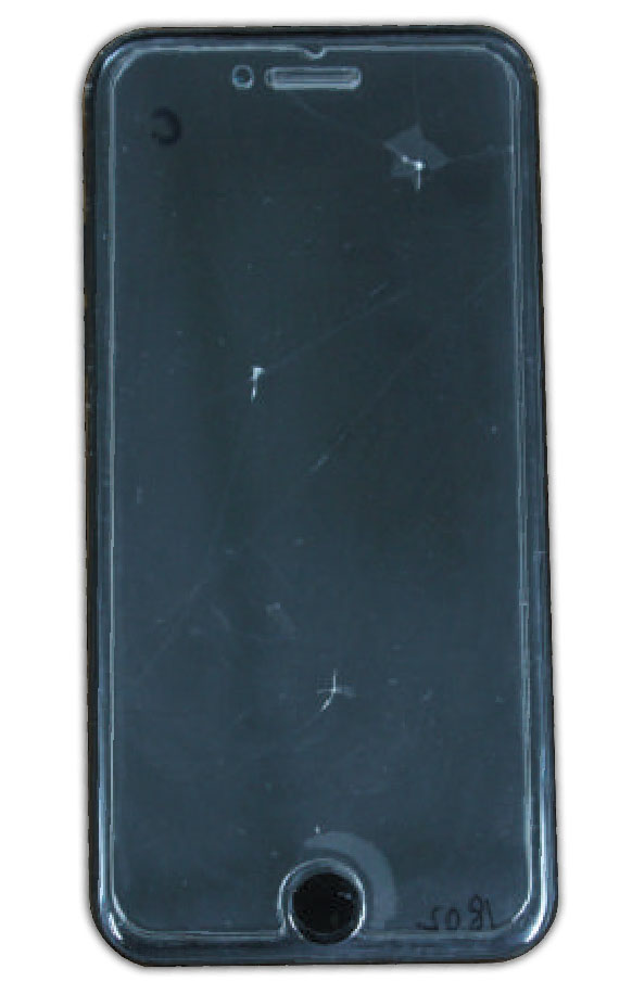
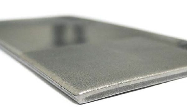
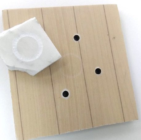
Bouldering grips used to compare surface roughness, pore morphology, and grip-related topography.

Why Use Non-Contact Profilometry for Climbing Hold Surface Analysis

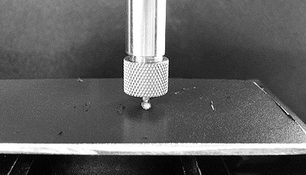
Climbing holds and rock-like surfaces can include deep pores, steep asperities, sharp valleys, and irregular texture. These features are difficult to measure accurately with contact-based profilometry because a physical stylus can lose contact, deform local surface features, or fail to reach narrow cavities.

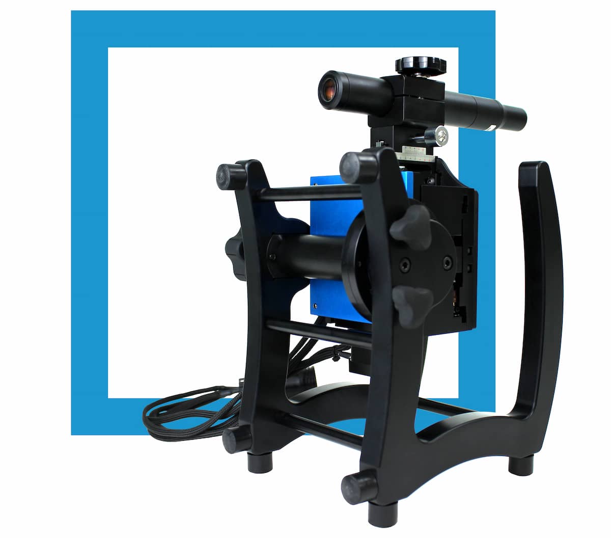
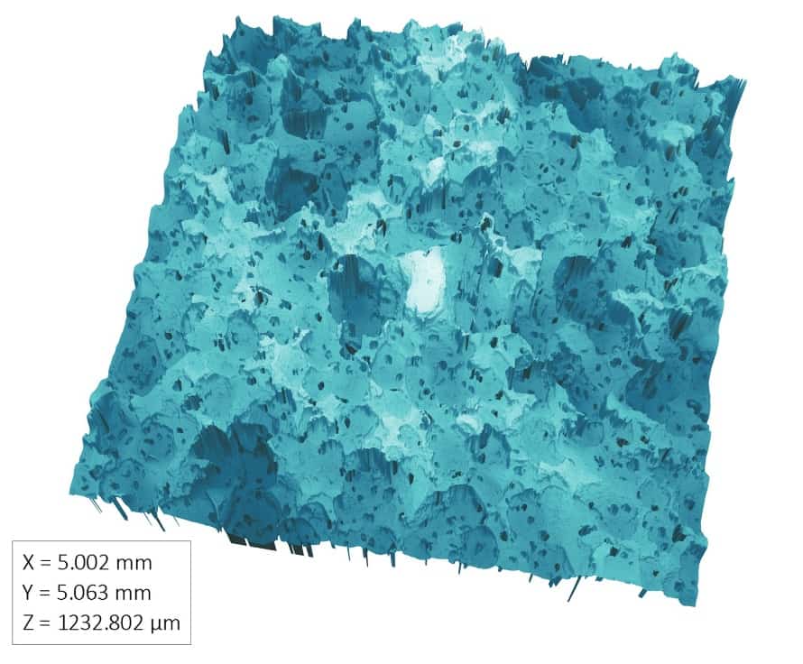
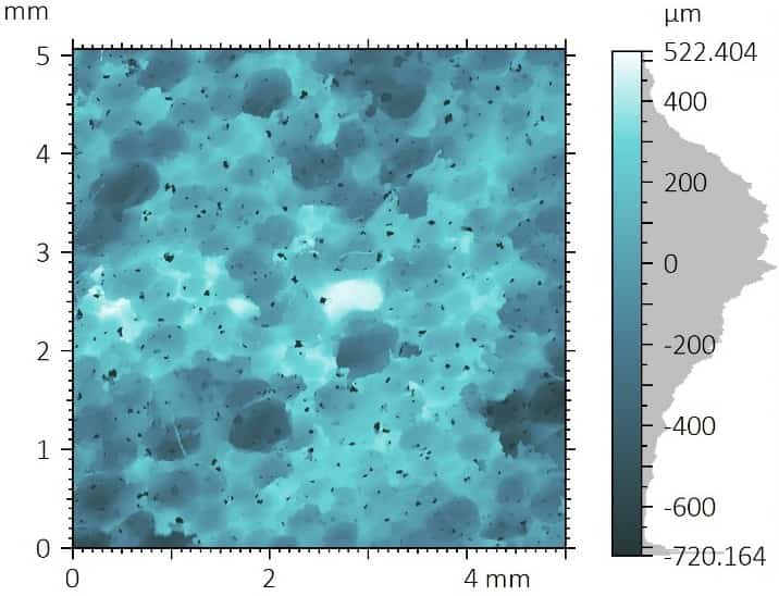
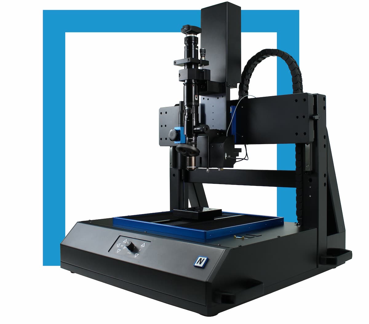
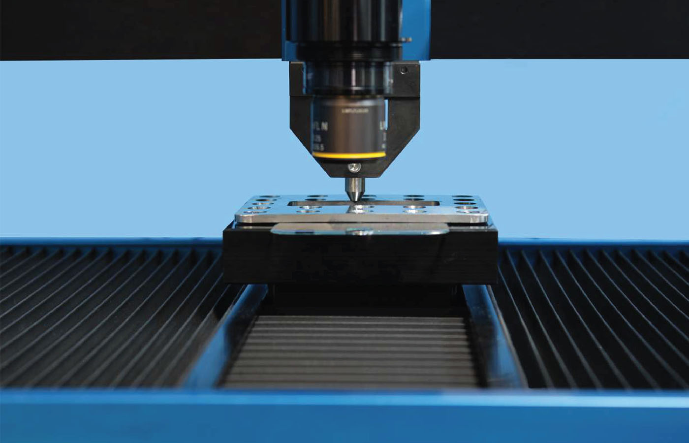
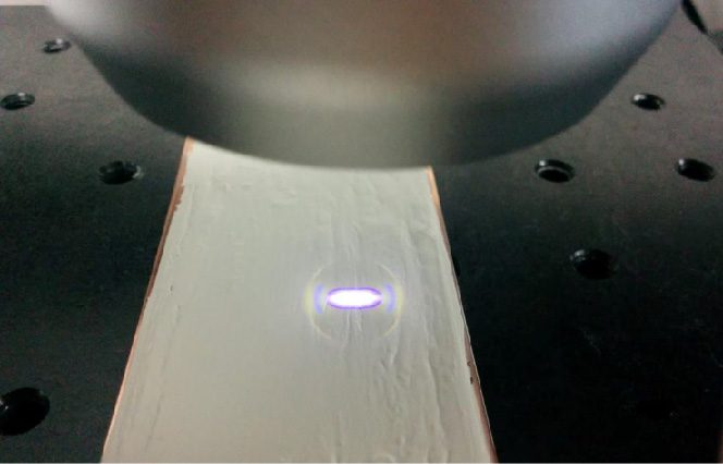
NANOVEA’s non-contact optical profilometry uses chromatic light technology to capture surface height data without touching the sample. This makes it suitable for reconstructing complex climbing hold topography, including deep nooks, pores, and surface flaws, while avoiding measurement artifacts caused by local plastic deformation.

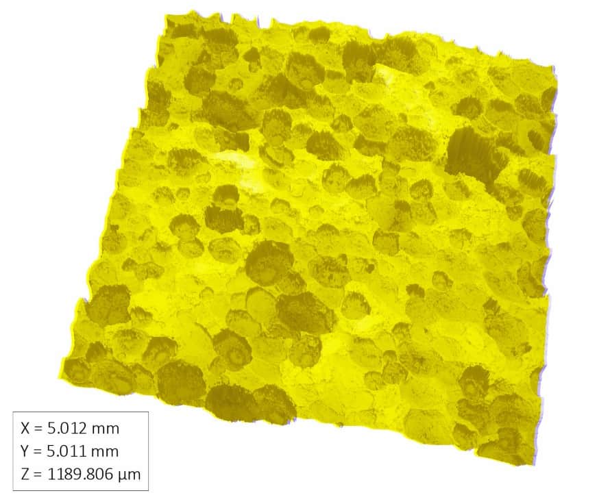
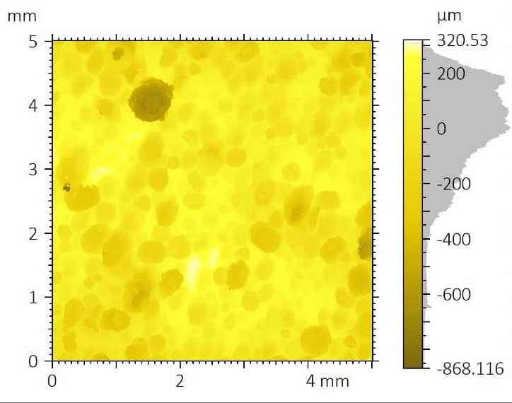
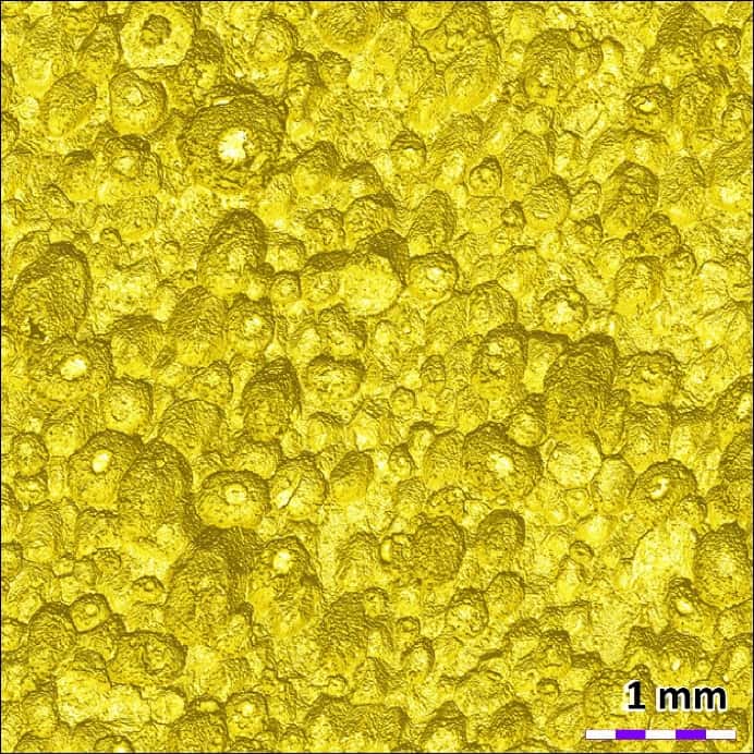
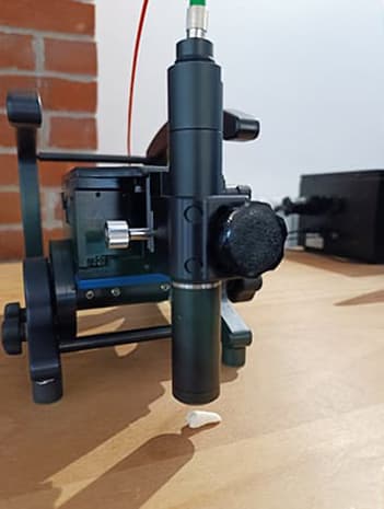
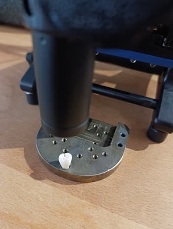
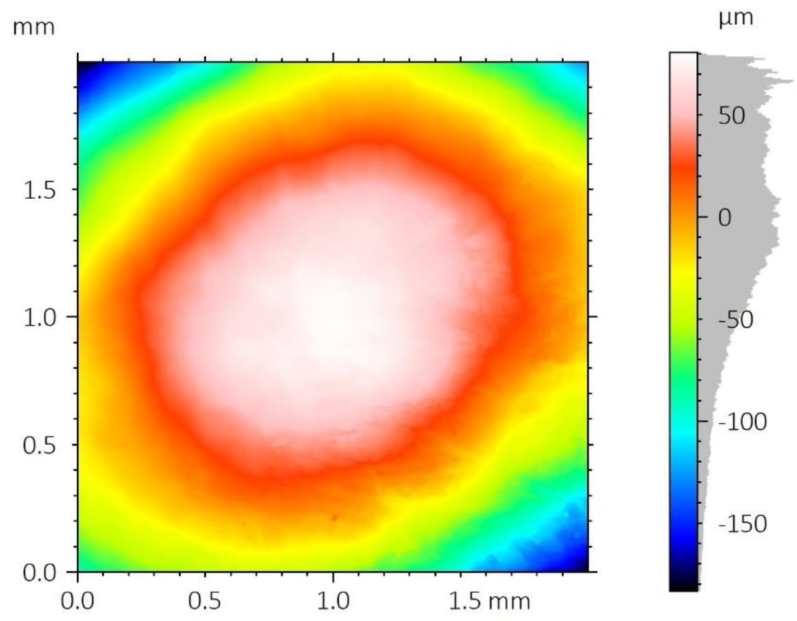
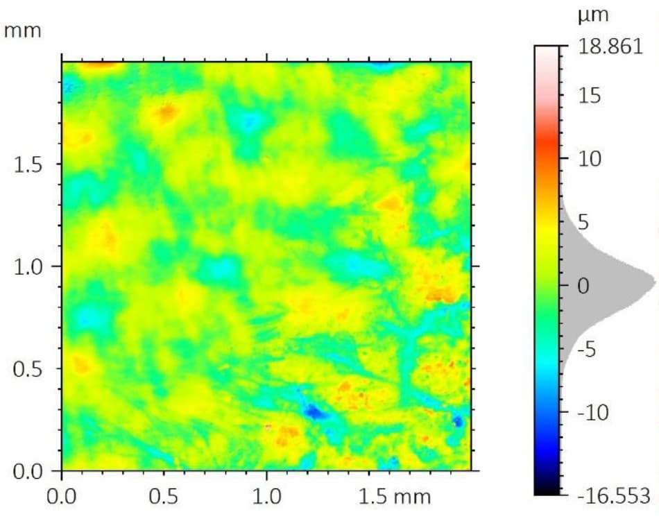
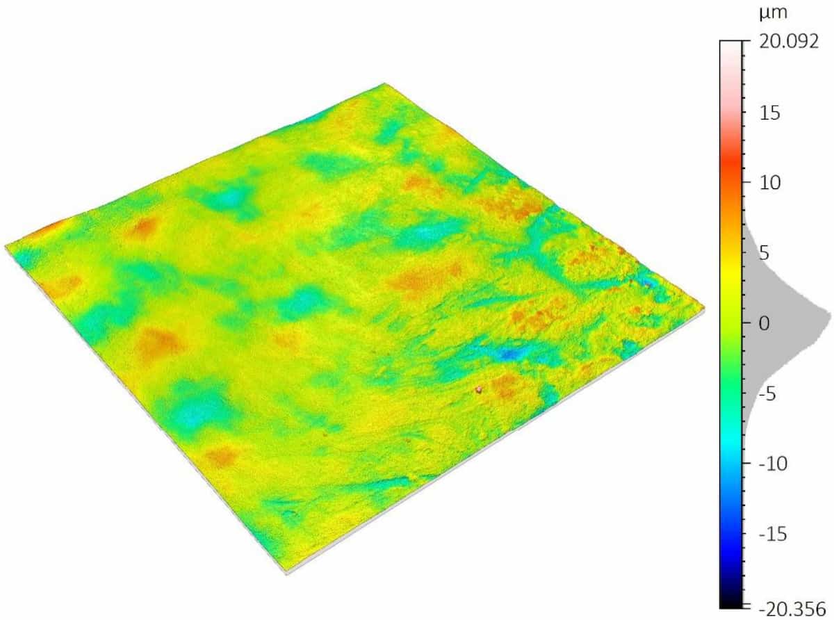
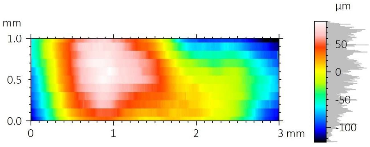
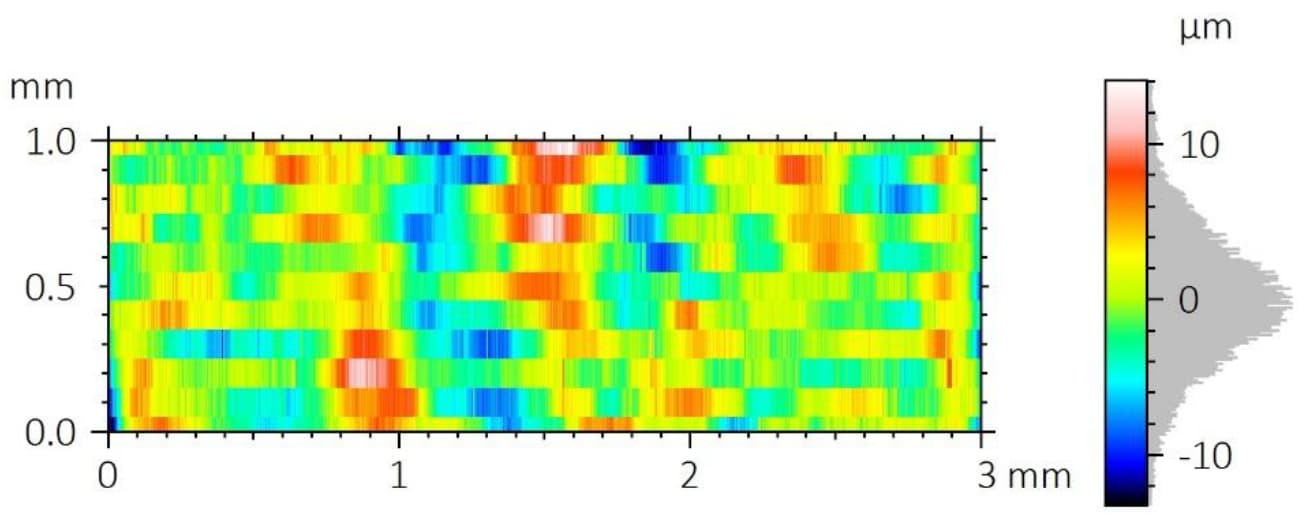
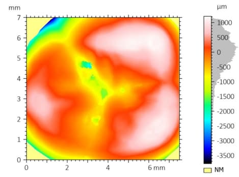
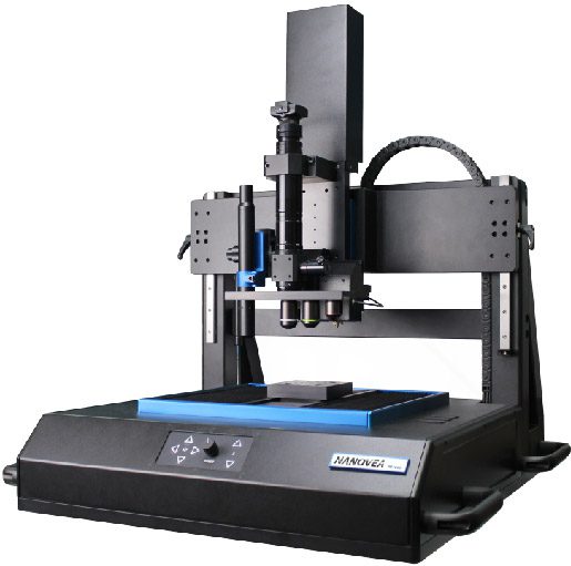
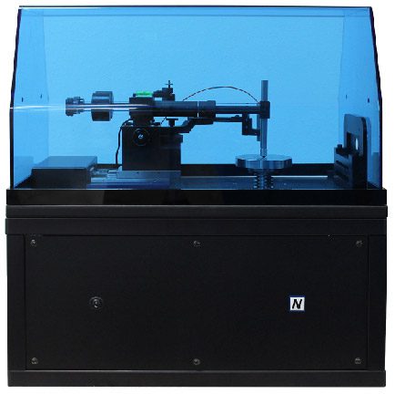
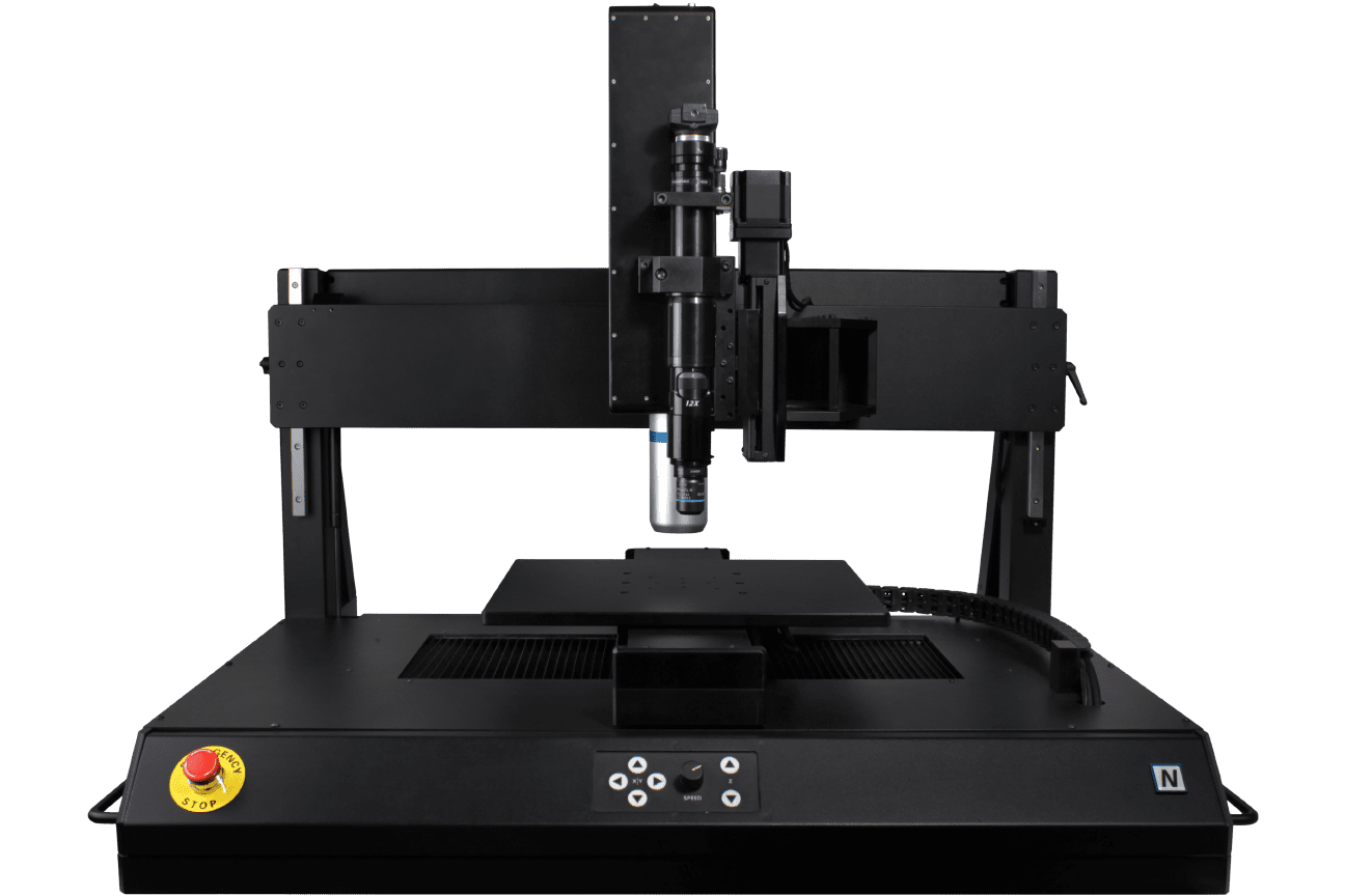
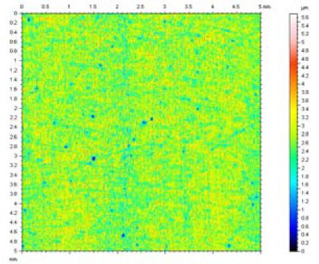
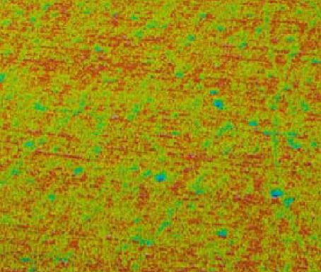
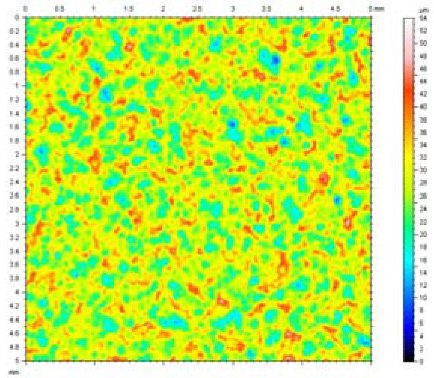
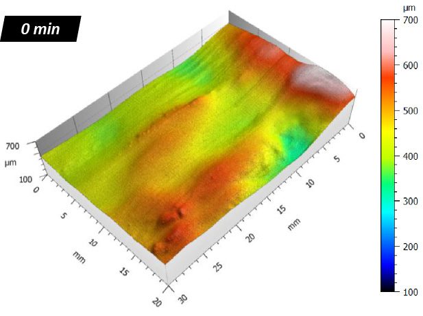
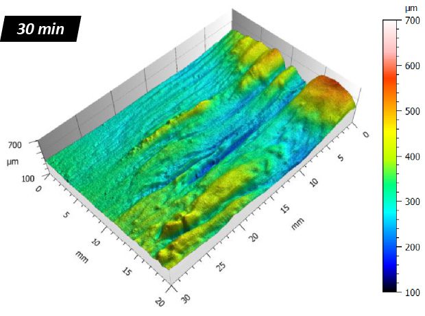
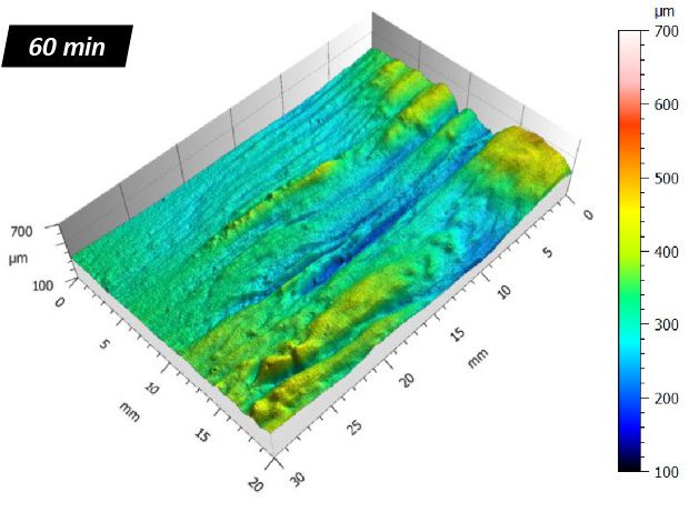
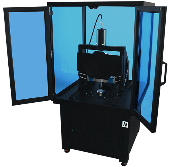
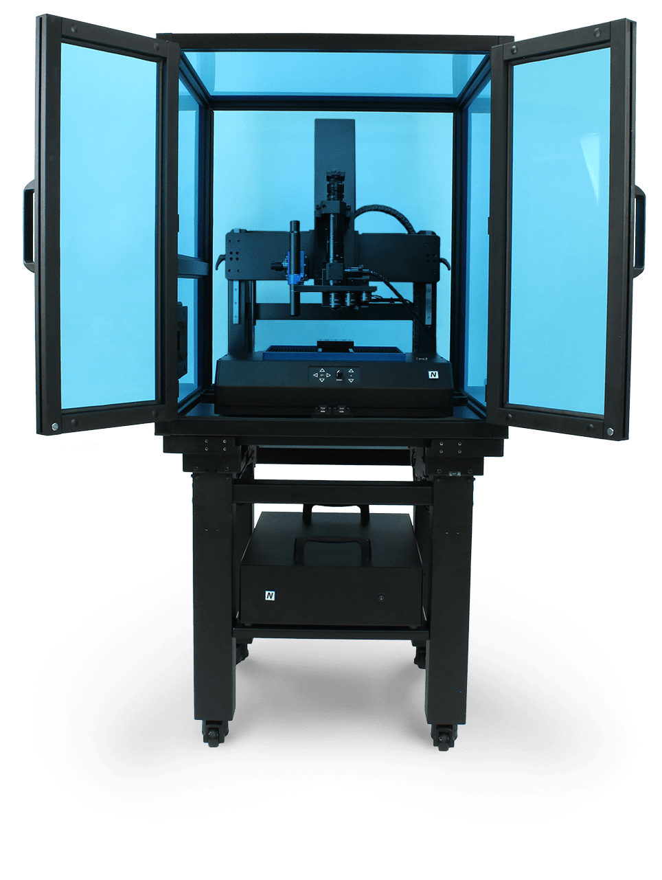
In this study, the NANOVEA JR25 Optical Profiler was used to measure two bouldering grips: a yellow block with a smoother, flatter surface and a green block with a rougher tactile texture. Both samples were scanned using a PS4-MG35 single-point optical sensor with a 3000 µm Z-range and a 4 µm acquisition step in X and Y.

Dual-frequency acquisition was used to reduce light sensor saturation from localized bright spots on the grip surfaces, allowing the profiler to capture roughness and pore morphology across the scanned areas.

Measurement Objective

The objective of this study was to demonstrate how non-contact 3D optical profilometry can be used to reconstruct and compare the surface roughness, topography, and pore morphology of climbing holds.

Two bouldering grip samples were analyzed: a yellow block with a smoother, flatter surface and a blue block with a rougher tactile texture and sharper grip features. The analysis focused on surface height variation, areal roughness parameters, pore coverage, pore size, pore depth, and functional surface behavior.

The NANOVEA JR25 Optical Profilometer measuring the climbing hold samples using an optical sensor.

Measurement Method

The NANOVEA JR25 Optical Profiler was used to measure the yellow and blue bouldering grip samples. Each surface was scanned with a PS4-MG35 single-point optical sensor with an enhanced 3000 µm Z-range, allowing the system to capture deep pores, sharp valleys, and irregular surface texture while maintaining a 4 µm acquisition step in X and Y.

Dual-frequency acquisition was used to reduce light sensor saturation from localized bright spots on the grip surfaces, improving data capture across rough, porous, and uneven areas.

NANOVEA JR25 Portable

Optical Profilometer

Test Parameters

Two bouldering grip samples were analyzed: a yellow grip with a smoother, flatter surface and a blue grip with a rougher tactile texture and sharper grip features. The analysis focused on surface height variation, areal roughness parameters, pore coverage, pore size, pore depth, and functional surface behavior.

Measurement Setting	Optical Profilometry Setup
Samples measured	Yellow and blue bouldering grip samples
Optical pen	PS4-MG35
Z-range	3000 µm
Scan area	5.00 mm × 5.00 mm
X-step size	4.00 µm
Y-step size	4.00 µm
Averaging	1
Measurement type	Direct
Acquisition mode	Dual frequency
Acquisition rate	100–400 Hz
Light intensity	100%

Table 1: Optical profilometry test conditions used to measure the bouldering grip samples.

Optical Profilometry Results

Yellow Grip Sample

Surface Roughness Analysis

The 3D rendering below shows the reconstructed surface topography of the yellow climbing grip sample.

A total least-squares plane was removed to study surface properties. The roughness filters S-Gaussian 2.5 µm was applied following ISO 25178 (1/2 cut-off removed at each side). However, the sharp density of pores and asperities and the elevated average roughness make the use of a Gaussian L-filter (8 mm cut off) inapplicable. Therefore, the primary surface was considered, and the roughness parameters are listed in the table below, alongside the 2D false-color map of the filtered surface.

ISO 25178-2 – Primary Surface
S-filter (λs): Gaussian, 2.5 µm, 1/2 cut-off
F-operation: [Workflow] Leveled (TLSPL)
Height Parameters
Sq	168.970	µm	Root-mean-square height
Ssk	-0.927		Skewness
Sku	4.117		Kurtosis
Sp	320.530	µm	Maximum peak height
Sv	868.116	µm	Maximum pit depth
Sz	1188.645	µm	Maximum height
Sa	132.953	µm	Arithmetic mean height

The average surface roughness Sa is 132.953 µm, whereas the peak-to-valley roughness, Sz amounts to 1188.645 µm. The surface morphology is skewed towards deep valleys (Ssk < 0, Sv > Sp), with a leptokurtotic (Sku > 3) distribution of peaks and valleys relative to the average plane.

The following picture shows a 2D photo-simulation of the area under artificial lighting, highlighting the region’s morphology.

Pore Morphology Analysis

A pore analysis was performed across the full scanned area using a semi-automated edge-detection algorithm. The analysis identified recessed surface features to quantify pore coverage, pore density, radius, void volume, and maximum depth.

The detected pore locations were then mapped across the scanned 5 mm × 5 mm area to evaluate pore coverage, density, and size distribution.

Information
Method	Circle detection
Features detected	Pores, recessed objects
Minimum detection diameter	0.150 mm
Maximum detection diameter	2.000 mm
Number of detected pores	206
Surface coverage	47.395%
Pore density	8.203 particles/mm²

Parameter	Unit	Mean	Std. Dev.	Min	Max
Global Statistics
Radius	mm	0.127	0.049	0.076	0.275
Void volume	µm³	4,724,770.705	6,748,143.925	23,594.172	4.422 × 10⁷
Maximum depth	µm	173.729	94.942	28.153	716.480

Pores covered nearly half of the yellow grip’s scanned surface, with a measured coverage of 47.395% and a pore density of 8.203 particles/mm². The detected pores and cracks were highly heterogeneous in size, volume, and depth, ranging from large crater-like features with a maximum radius of 0.275 mm and void volume above 4.4 × 10⁷ µm³ to smaller pores with a minimum radius of 0.076 mm and void volume of 23,594.172 µm³. This uneven pore distribution is reflected in the large standard deviation measured for void volume and maximum depth.

Functional Surface Parameters (Abbott-Firestone curve)

The Abbott-Firestone curve shows the cumulative areal material distribution of the yellow climbing grip sample. This analysis defines functional surface parameters including Sk, Spk, and Svk according to ISO 25178-2.

Information
Standard	ISO 25178-2
Parameter	Value	Unit
Sk	409.738	µm
Spk	45.480	µm
Svk	233.446	µm
Smrk1	3.976	%
Smrk2	85.005	%

The chart below shows the peak-valley distribution from the mean plane based on the functional parameters derived from the Abbott-Firestone curve. Valleys are shown in purple, the mean plane in green, and peaks in orange.

Information
1st threshold	Height – c1: 229.209 µm
2nd threshold	Height – c2: -180.424 µm
Parameters	Unit
Projected area (in %)	%	14.995	81.029	3.976
Projected area	mm²	3.772	20.381	1.000
Volume of material (in %)	%	97.451	48.100	0.973
Volume of material	µm³	1.684 × 10¹⁰	4.956 × 10⁹	2.275 × 10⁷

The yellow grip sample shows a dominant mean-plane region with scattered recessed pores and a smaller population of raised peaks. This indicates a surface texture characterized mainly by average-sized pores distributed across the scanned area.

Blue Grip Sample

Surface Roughness Analysis

The 3D rendering below shows the reconstructed surface topography of the blue climbing grip sample.

A total least-squares plane was removed to evaluate the blue grip’s surface properties. An S-Gaussian 2.5 µm roughness filter was applied following ISO 25178, with 1/2 cut-off removed at each side.

Because of the dense pores, asperities, and elevated average roughness, a Gaussian L-filter with an 8 mm cut-off was not applied. The primary surface was used for roughness analysis, with the roughness parameters listed alongside the 2D false-color map of the filtered surface.

ISO 25178-2 – Primary Surface
S-filter (λs): Gaussian, 2.5 µm, 1/2 cut-off
F-operation: [Workflow] Leveled (TLSPL)
Height Parameters
Sq	211.440	µm	Root-mean-square height
Ssk	-0.682		Skewness
Sku	3.672		Kurtosis
Sp	522.404	µm	Maximum peak height
Sv	720.164	µm	Maximum pit depth
Sz	1242.568	µm	Maximum height
Sa	166.719	µm	Arithmetic mean height

The blue grip sample had an average surface roughness, Sa, of 166.719 µm and a peak-to-valley roughness, Sz, of 1242.568 µm. The negative skewness value, Ssk < 0, indicates that the surface morphology is skewed toward deep valleys, while Sv > Sp shows that the maximum pit depth exceeded the maximum peak height.

The kurtosis value, Sku > 3, indicates a leptokurtotic height distribution, meaning the blue grip surface contains sharper or more extreme peaks and valleys relative to the average plane.

The 2D photo simulation below highlights the blue climbing grip’s surface morphology under artificial lighting.

Pore Morphology Analysis

The detected pore locations were mapped across the scanned 5 mm × 5 mm area to evaluate pore coverage, density, and size distribution.

Information
Method	Circle detection
Features detected	Pores, recessed objects
Minimum detection diameter	0.040 mm
Maximum detection diameter	2.000 mm
Number of detected pores	794
Surface coverage	24.208%
Pore density	31.355 particles/mm²

Parameter	Unit	Mean	Std. Dev.	Min	Max
Global Statistics
Radius	mm	0.035	0.035	0.020	0.218
Void volume	µm³	821,872.849	2,495,310.021	11,009.819	2.929 × 10⁷
Maximum depth	µm	476.053	305.830	16.132	1044.045

Pores covered 24.208% of the blue grip’s scanned surface, with a pore density of 31.355 particles/mm². The detected pores and cracks were highly heterogeneous in size, volume, and depth, ranging from large crater-like features with a maximum radius of 0.218 mm and void volume greater than 2.9 × 10⁷ µm³ to small pores with a minimum radius of 0.020 mm and void volume of approximately 1.1 × 10⁴ µm³.

This uneven distribution is reflected in the large standard deviation measured for void volume and maximum depth. The pore distribution is bimodal, with one population of fine, deep pores and another population of larger crater-like valleys.

Functional Surface Parameters (Abbott-Firestone curve)

The Abbott-Firestone curve shows the cumulative areal material distribution of the blue climbing grip sample. This analysis defines functional surface parameters including Sk, Spk, and Svk according to ISO 25178-2.

Information
Standard	ISO 25178-2
Parameter	Value	Unit
Sk	522.359	µm
Spk	117.670	µm
Svk	295.209	µm
Smrk1	6.122	%
Smrk2	87.456	%

Information
1st threshold	Height – c1: 283.646 µm
2nd threshold	Height – c2: -238.619 µm
Parameters	Unit
Projected area (in %)	%	12.544	81.334	6.122
Projected area	mm²	3.182	20.629	1.553
Volume of material (in %)	%	96.079	48.546	1.514
Volume of material	µm³	1.151 × 10¹⁰	6.431 × 10⁹	9.142 × 10⁷

The blue grip sample shows a dominant mean-plane region with fine, deep pores distributed across the surface and localized peak features. Compared with the yellow grip, the blue grip contains a higher projected peak area and a bimodal pore structure, combining fine recessed pores with larger crater-like valleys.

Conclusion

In this application, the NANOVEA JR25 Non-Contact Optical Profiler was used to measure the surface roughness, topography, and pore morphology of yellow and blue bouldering grip samples.

Topographic analysis showed that both grip samples had high surface roughness, with Sa values above 100 µm and Sz values above 1000 µm. Both surfaces also showed an asymmetric height distribution skewed toward valleys, indicating that recessed features played a major role in the measured surface morphology.

The yellow grip sample showed higher pore coverage, with pores covering 47.395% of the scanned surface. Its surface was mainly characterized by average-sized pores distributed across the measured area.

The blue grip sample showed lower pore coverage at 24.208%, but a much higher pore density of 31.355 particles/mm². Its pore distribution was bimodal, with a population of fine, deep pores and a separate population of larger crater-like valleys.

These results show how non-contact 3D optical profilometry can quantify climbing hold surface features that are difficult to evaluate from visual inspection alone, including roughness, pore coverage, pore depth, surface height distribution, and functional topography. The blue grip’s higher porosity and bimodal pore structure make it more likely to absorb moisture and chalk at the contact interface, while its elevated roughness and surface morphology support stable friction for shoe rubber and finger contact. The yellow grip’s lower roughness and flatter profile suggest it is better suited for use as a foothold in slab climbing, where broad surface contact matters more than deep textural engagement.

Frequently Asked Questions About Climbing Hold Surface Roughness

What is climbing hold surface roughness?

Climbing hold surface roughness describes the height variation, texture, pores, asperities, and valleys present on the surface of a climbing grip. These features can influence contact behavior between the hold, shoe rubber, skin, chalk, and moisture.

How can climbing hold surface roughness be measured?

Climbing hold surface roughness can be measured using non-contact 3D optical profilometry. This method reconstructs the surface topography and calculates areal roughness parameters such as Sa, Sz, Sp, Sv, Ssk, and Sku without touching or deforming the sample.

Why use non-contact optical profilometry for climbing hold analysis?

Non-contact optical profilometry is useful for climbing hold analysis because climbing grips can contain deep pores, sharp valleys, rough asperities, and irregular surface texture. A contact stylus may lose contact, fail to reach recessed features, or introduce artifacts on complex surfaces.

What does Sa mean in surface roughness analysis?

Sa is the arithmetic mean height of a surface and is commonly used to describe average areal surface roughness. In this app note, both climbing grip samples showed high Sa values above 100 µm, indicating strongly textured surfaces.

What does Sz mean in optical profilometry results?

Sz is the maximum height of the measured surface, calculated from the highest peak to the deepest valley. In climbing hold surface roughness analysis, Sz helps describe the full vertical range of the grip’s surface texture.

Why is pore morphology important for climbing grips?

Pore morphology can affect how a climbing grip interacts with chalk, sweat, humidity, skin, and shoe rubber. Measuring pore coverage, density, depth, and volume helps quantify surface features that are difficult to evaluate by visual inspection alone.

Need Reliable Surface Roughness Analysis?

Stent Coating Adhesion and Delamination Analysis Using Nano Scratch Testing

Application Note | Stent Coating Adhesion Testing

Stent Coating Adhesion and Delamination Analysis Using Nano Scratch Testing

Quantifying Coating Failure and Adhesion Performance on Drug-Eluting Stents

Research & Experimental Testing

Duanjie Li, PhD

Visual Design & Editorial

Andrew Shore

Introduction

Blood is carried through arteries from the heart to the rest of the body. Any weakening or blockage of these vessels can pose significant health risks and may become life-threatening. A stent is a small mesh tube inserted into the lumen of a blood vessel to treat narrowed or weakened arteries. Stent implantation is now a widely used procedure to support the arterial wall and restore blood flowᶦ.

Metal stent mesh geometry illustrating the structural complexity of vascular implant design.

Why coating adhesion matters in drug-eluting stents

Drug-eluting stents represent a major advancement in stent technology. They incorporate a biodegradable, biocompatible polymer coating that enables controlled drug release at the arterial site, helping to inhibit intimal thickening and reduce the risk of restenosisᶦᶦ.

A critical concern in these systems is the delamination of the polymer coating from the metallic stent substrate. This coating carries the drug-eluting layer, and its adhesion directly impacts device performance and reliability.

To improve coating adhesion, stents are often designed with complex geometries. In this study, the polymer coating is located at the bottom of grooves within the stent mesh. This configuration presents a significant challenge for adhesion measurement.

A reliable method is required to quantitatively evaluate the interfacial strength between the polymer coating and the metal substrate. The small diameter of the stent mesh, comparable to a human hair, combined with its three-dimensional geometry, requires:

ultrafine X-Y positioning accuracy
precise control of applied load
accurate depth measurement during testing

ℹ️ Learn more about nanoindentation and scratch testing lab services for coating adhesion and failure analysis.

Measurement Method

Nano scratch testing is performed using the NANOVEA PB1000 Mechanical Tester, in Nano Scratch Mode, to evaluate the cohesive and adhesive strength of the polymer coating on the metal mesh of stent samples.

Controlled scratch measurements are carried out on stent geometries with dimensions comparable to a human hair, enabling precise evaluation of coating adhesion on complex stent structures.

NANOVEA PB1000 Advanced

Mechanical Tester

Test Conditions

1. Regular Stent Samples

The stent is fixed on the sample stage, with a support wire inserted inside the stent tube to ensure stability during nano scratch testing. The NANOVEA Mechanical Tester is used to perform nano scratch measurements using the parameters summarized in Table 1, to evaluate the cohesive and adhesive strength of the polymer coating on the metal substrate.

Parameter	Value
Load type	Progressive
Initial load	0.05 mN
Final load	300 and 100 mN
Sliding speed	0.5 mm/min
Sliding distance	0.5 mm
Indenter geometry	Conical
Indenter material (tip)	Diamond
Indenter tip radius	20 µm
Temperature	24°C (room)

Table 1: Test parameters for nano scratch measurements on regular stent samples

2. Grooved Stent Samples

The SEM image in Fig. 1 shows the cross-section of the stent sample. The stent features a groove with a depth of approximately 30 µm. The polymer coating, with a thickness of 10.8 µm, is located at the bottom of the groove.

Standard 60° conical diamond tips are not sharp enough to reach the bottom of the groove without contacting the sidewalls. Therefore, a sharper 40° conical diamond tip is used in this study (Fig. 2).

Nano scratch measurements are performed using the parameters summarized in Table 2.

Parameter	Value
Load type	Progressive
Initial load	0.1 mN
Final load	300 mN
Loading rate	300 mN/min
Scratch length	0.25 mm
Scratch speed	0.25 mm/min
Indenter geometry	40° cone
Indenter material (tip)	Diamond
Indenter tip radius	5 µm

Table 2: Test parameters for nano scratch measurements on grooved stent samples

Fig. 1: SEM cross-section of a grooved stent showing polymer coating located at the bottom of the groove, highlighting the challenge of coating adhesion measurement in recessed geometries.

Fig. 2: Schematic of a 40° conical diamond tip designed for nano scratch testing inside stent grooves, enabling accurate adhesion measurement without sidewall interference.

Results and Discussion

The stent mesh has a diameter of approximately 100 μm, comparable to a human hair. Precise positioning is therefore critical to ensure the scratch test is performed at the center of the stent mesh. The NANOVEA Mechanical Tester provides X–Y positioning accuracy down to 0.25 μm, enabling accurate test placement under the integrated optical microscope.

1. Regular Stent Samples

Nano scratch testing is performed with a progressively increasing load up to 300 mN. The full scratch track on the stent is shown in Fig. 3a, while failure behavior at different stages is presented in Fig. 3b and 3c.

Two critical loads are identified:

Lc1: the load at which the first visible damage appears on the coating
Lc2: the load at which the coating is fully removed and the substrate is exposed

The evolution of coefficient of friction (COF) and penetration depth is shown in Fig. 4, providing insight into the progression of coating failure during the test.

The first signs of coating damage appear at Lc1 ≈ 14.5 mN. As the applied load increases, the diamond tip progressively penetrates the polymer coating, resulting in a wider and deeper scratch track. During this phase, the COF increases from approximately 0.05 to 0.7.

At Lc2 ≈ 78.1 mN, the coating is fully delaminated from the metal substrate. Beyond this point, as the load continues to increase, both COF and penetration depth remain relatively stable due to the mechanical support of the underlying metal substrate.

(a) Full Scratch Track

(b) Lc1 ≈ 14.5 mN

Fig. 3: Nano scratch track on a stent coating under progressively increasing load, showing (a) full scratch path, (b) initial coating failure at Lc1 ≈ 14.5 mN, and (c) complete coating delamination at Lc2 ≈ 78.1 mN.

Fig. 4: Evolution of coefficient of friction (COF) and penetration depth during nano scratch testing of a stent coating under progressively increasing load, showing the progression of coating failure and transition to substrate support.

Failures during nano scratch testing up to a maximum load of 300 mN occur at critical loads below 100 mN. To enable a more quantitative comparison of coating performance, additional tests are performed with a maximum load of 100 mN on two stent samples, referred to as Sample 1 and Sample 2.

Fig. 5 compares the scratch tracks of Sample 1 and Sample 2 after nano scratch testing. Sample 1 exhibits the first sign of coating damage at a critical load of Lc1 ≈ 13.2 mN, while Sample 2 shows initial failure at a higher load of Lc1 ≈ 21.1 mN.

Coating delamination occurs at 62.5 mN for Sample 1. In contrast, the coating on Sample 2 remains intact throughout the test, continuing to protect the metal substrate under the same loading conditions.

This behavior is further reflected in the evolution of coefficient of friction (COF) and penetration depth, as shown in Fig. 6. When the diamond tip penetrates through the coating and contacts the metal substrate in Sample 1, the COF reaches a peak while the penetration depth decreases due to the increased stiffness of the underlying substrate.

(a) Sample 1 – Early Coating Failure

(b) Sample 2 – Improved Coating Integrity

Fig. 5: Comparison of nano scratch tracks for two stent coatings, showing (a) early coating failure and delamination in Sample 1, and (b) improved coating integrity in Sample 2 under the same loading conditions.

Fig. 6: Comparison of coefficient of friction (COF) and penetration depth for Sample 1 and Sample 2 during nano scratch testing, showing earlier substrate contact and higher friction response in Sample 1, indicating weaker coating adhesion.

2. Grooved Stent Samples

As shown in Fig. 1 and Fig. 7, the grooved stent mesh has a diameter of approximately 90 μm, comparable to a human hair. The groove has a width of ~50 μm and a depth of 30 μm. This geometry presents a significant challenge for nano scratch testing, particularly for evaluating coating adhesion at the bottom of the groove.

Precise positioning is critical to locate the scratch test within the groove. The nano scratch test is performed with a progressively increasing load up to 300 mN. The full scratch tracks of grooved stent Samples 3 and 4 are compared in Fig. 7.

The critical load Lc is defined as the load at which the coating fails and the substrate becomes exposed. The evolution of normal load and penetration depth, shown in Fig. 8, provides further insight into the progression of coating failure during testing.

As the applied load increases, the diamond tip progressively penetrates the polymer coating, resulting in a deeper scratch track. When the critical load Lc is reached, the coating delaminates from the metal substrate.

Sample 3 exhibits coating failure at Lc ≈ 126 mN, while Sample 4 fails at a higher load of Lc ≈ 173 mN. This difference indicates stronger adhesion of the coating in Sample 4.

The measured critical loads enable quantitative comparison of coating adhesion performance. Under the same testing conditions, the coating on Sample 4 demonstrates higher resistance to delamination, making it the better-performing candidate in this study.

(d) Sample 4 – Higher Adhesion in Groove (Lc ≈ 173 mN)

Fig. 7: Nano scratch tracks inside stent grooves for Samples 3 and 4, showing (c) coating failure at Lc ≈ 126 mN in Sample 3 and (d) higher adhesion with delayed failure at Lc ≈ 173 mN in Sample 4.

(a) Sample 3 – Earlier Coating Failure (Lc ≈ 126 mN)

(b) Sample 4 – Delayed Failure and Higher Adhesion (Lc ≈ 173 mN)

Fig. 8: Evolution of normal load and penetration depth during nano scratch testing inside stent grooves for Samples 3 and 4, showing earlier coating failure in Sample 3 and delayed failure at higher load in Sample 4. The vertical green line indicates the critical load (Lc) where coating delamination occurs.

Conclusion

This study demonstrates the ability of the NANOVEA Mechanical Tester to quantitatively evaluate the cohesive and adhesive strength of polymer coatings on both regular and grooved stent geometries using nano scratch testing.

The recessed geometry of the stent grooves, approximately 50 μm wide and 30 μm deep, presents a significant challenge for coating adhesion measurement. The high X–Y positioning accuracy of 0.25 μm enables precise placement of the scratch test within these confined regions, allowing direct evaluation of coating performance where failure is most critical.

By applying a controlled, progressively increasing load, critical loads associated with coating failure can be identified and compared across samples. This approach enables reliable differentiation of coating adhesion performance and interfacial integrity, even on small, complex stent structures.

References

[I] http://www.nhlbi.nih.gov/health/health-topics/topics/stents
[II] http://www.scielo.org.mx/scielo.php?script=sci_arttext&pid=S1405-99402006000300008

Frequently Asked Questions About Stent Coating Adhesion Testing

What is stent coating adhesion testing?

Stent coating adhesion testing evaluates how strongly a polymer coating is bonded to the metal substrate of a stent. Techniques such as nano scratch testing quantify the load at which coating damage and delamination occur, providing measurable indicators of adhesion strength.

What is critical load (Lc) in nano scratch testing?

Critical load (Lc) is the applied load at which a coating fails during a scratch test.

Lc1 corresponds to the first visible damage in the coating
Lc2 indicates complete coating removal and exposure of the substrate

These values are used to quantify and compare coating adhesion performance.

Why is coating adhesion important in drug-eluting stents?

Coating adhesion directly affects the reliability of drug-eluting stents. Poor adhesion can lead to coating delamination, which may compromise controlled drug release and increase the risk of device failure.

How do you measure coating adhesion inside stent grooves?

Measuring adhesion inside stent grooves requires high positioning accuracy and appropriate indenter geometry. Nano scratch testing with sharp diamond tips allows access to recessed coating regions, enabling direct evaluation of adhesion within complex stent geometries.

What does coefficient of friction (COF) indicate in scratch testing?

The coefficient of friction (COF) reflects changes in surface interaction during the scratch test. A sudden increase in COF often indicates coating failure and contact between the indenter and the underlying metal substrate.

How can nano scratch testing compare different coating formulations?

Nano scratch testing enables direct comparison of coatings by measuring critical loads under controlled conditions. Higher critical loads indicate stronger adhesion and improved resistance to delamination, allowing selection of better-performing coating systems.

Need Reliable Stent Coating Adhesion Testing?

Dental Surface Roughness Measurement & 3D Tooth Topography

Application Note | Dental Surface Characterization

Dental Surface Roughness Measurement and Full 3D Tooth Topography

Surface Roughness Analysis Using Non-Contact Optical Profilometry

Prepared by

Walter Alabiso, PhD; Davide Morrone, MPhys; Andrew Shore, MA

Introduction

The ability to accurately characterize tooth surfaces, including micro-roughness and 3D surface topography at the nanometer scale, enables advanced research and applications in orthodontics and dental materials science. Non-contact optical profilometry provides a precise method for measuring dental surface roughness and analyzing tooth surface morphology without damaging delicate structures. These measurements support the development of composite dental materials that replicate the natural surface roughness of enamel, as well as the design and fabrication of patient-specific dental casts and restorative components.

Low surface roughness plays a primary role in limiting bacterial adhesion and plaque formation, thereby reducing the risk of cavities. An increase in average roughness (Ra) above 2 µm leads to a steep increase in biofilm formation in vivo.¹ An Ra of 0.2 µm is considered the threshold value below which no further reduction in bacterial adhesion can be expected.²

Reconstruction of the tooth’s 3D surface topography enables the fabrication of dental casts, which are essential for accurate diagnosis, treatment planning, and the fabrication of dental appliances.

Non-Contact Optical Profilometry for Dental Surface Analysis

The present study illustrates the potential of NANOVEA’s high-precision non-contact optical profilometers for dental surface roughness measurement and 3D tooth topography analysis. Chromatic Light technology offers significant advantages over classical touch probe techniques. It acquires data points from deep crevices and complex geometries without introducing measurement errors or artifacts caused by local plastic deformation and without requiring extensive data manipulation.

Compared to focus variation systems, single-point optical sensing provides superior lateral and height accuracy, with X/Y resolution below 0.5 µm, maximum vertical resolution of 1.9 nm, and the ability to measure surface angles up to 87°. The technique is effective on transparent, opaque, specular, diffusive, polished, and rough dental surfaces, making it well suited for comprehensive dental surface characterization.

ℹ️ Learn more about non-contact optical profilometry and surface roughness measurement services.

Measurement Method

In this application, the NANOVEA JR25 Non-Contact Optical Profiler was used to analyze the surface roughness and 3D surface topography of an adult human molar previously affected by tooth decay. The side of the tooth was scanned using a PS2–MG140 single-point optical sensor to measure surface roughness parameters over a defined region of interest and along multiple line profiles.

The crown of the tooth was then scanned and reconstructed using a PS5–MG35 single-point optical sensor, which is suited for larger-area acquisition and full 3D tooth topography measurement.

NANOVEA JR25 Portable
Optical Profilometer

Surface Measurement Using NANOVEA Optical Profilometer

Surface roughness measurements were performed on the lateral side of the molar crown, followed by full 3D reconstruction of the crown surface. Separate single-point optical sensors were used to optimize measurement accuracy for both localized roughness analysis and large-area surface topography acquisition.

PS2 – MG140

Surface roughness analysis by area and parallel line profiles on the side of the tooth’s crown.

PS5 – MG35

Full 3D surface reconstruction of the tooth’s crown.

Measurement Parameters

The following measurement parameters were used for localized surface roughness analysis and full 3D surface reconstruction of the molar crown using NANOVEA single-point optical sensors.

Parameter	Roughness Analysis (Area)	Roughness Analysis (Profiles)	Full 3D Reconstruction
Optical Pen	PS2-MG140	PS2-MG140	PS5-MG35
Z-Range [µm]	300	300	10000
X-Distance [mm]	2.00	3.00	7.50
X-Step Size [µm]	1.70	1.70	10.00
Y-Distance [mm]	2.00	1.00	7.00
Y-Step Size [µm]	1.70	100.00	10.00
Averaging (Avg)	1	1	1
Measurement Type	Direct	Direct	Direct
Acquisition Mode	Single Frequency	Single Frequency	Dual Frequency
Acquisition Rate [Hz]	200	200	100–400
Light Intensity [%]	100	100	100

Optical Profilometry Results

Surface Roughness Analysis (Area)

The PS2 single-point optical sensor was used to investigate fine surface features on the side of the tooth. The image below shows a false-color 2D surface map of the scanned region obtained by non-contact optical profilometry.

A least-squares degree-8 polynomial form removal was applied to isolate the surface roughness component. The roughness filters S-Gaussian 2.5 µm and L-Gaussian 0.8 mm were then applied according to ISO 25178. The resulting filtered surface and corresponding roughness parameters are presented below.

ISO 25178 – Roughness (S-L)
S-filter (λs): Gaussian, 2.5 µm
F: [Workflow] Form removed (LS-poly 8)
L-filter (λc): Gaussian, 0.8 mm
Height Parameters
Sq	2.433	µm	Root-mean-square height
Ssk	-0.102		Skewness
Sku	3.715		Kurtosis
Sp	18.861	µm	Maximum peak height
Sv	16.553	µm	Maximum pit depth
Sz	35.414	µm	Maximum height
Sa	1.888	µm	Arithmetic mean height

The average surface roughness Sa is 1.888 µm, while the peak-to-valley height Sz reaches 35.414 µm.

A 3D surface rendering of the filtered area is shown below for visualization.

Roughness Analysis (Profiles)

Surface roughness profiles were measured using a series of 11 parallel line scans along the X direction on the side of the tooth. The false-color 2D surface map of the raw scan is shown below.

The surface form was removed using a least-squares 8-degree polynomial prior to applying the metrological filters, leaving the residual surface shown below.

A statistical analysis of the measured surface roughness profiles reveals the following line roughness parameters.

		Description	Mean	Std dev	Min	Max
ISO 4287 – Roughness (S-L)
F: None
S-filter (λs): Gaussian, 2.5 µm
L-filter (λc): Gaussian, 0.8 mm
Evaluation length: All λc (3)
Amplitude Parameters – Roughness Profile
Rp	µm	Maximum peak height of the roughness profile	5.683	0.761	4.315	6.610
Rv	µm	Maximum valley depth of the roughness profile	6.242	1.009	4.701	8.438
Rz	µm	Maximum height of roughness profile	11.925	1.676	9.123	15.048
Ra	µm	Arithmetic mean deviation of the roughness profile	2.063	0.297	1.710	2.629
Rq	µm	Root-mean-square (RMS) deviation of the roughness profile	2.523	0.361	2.057	3.175

F: None

S-filter (λs): Gaussian, 2.5 µm

L-filter (λc): Gaussian, 0.8 mm

Evaluation length: All λc (3)

The value of Ra is consistent with the Sa value extracted from the surface area measurement.

Different metrological filters can be applied to distinguish between macroscopic waviness and microscopic surface roughness. For example, a coarser filter cut-off, such as the 8 mm cut-off used with the Robust Gaussian order-2 filter, produces a smoother waviness profile (red) that is less sensitive to sharp local variations and follows the original surface profile more loosely.

Alternatively, a finer cut-off (e.g., 0.08 mm) enables the analysis of micro-roughness by removing the waviness component that follows the original profile at a larger scale, leaving the finer surface roughness features of the tooth visible.

The microroughness analysis obtained using a 0.08 mm L-Gaussian filter is presented below.

		Description	Mean	Std dev	Min	Max
ISO 4287 – Roughness (S-L)
F: None
S-filter (λs): Gaussian, 2.5 µm
L-filter (λc): Gaussian, 0.08 mm
Evaluation length: All λc (37)
Amplitude Parameters – Roughness Profile
Rp	µm	Maximum peak height of the roughness profile	1.582	0.122	1.342	1.748
Rv	µm	Maximum valley depth of the roughness profile	1.466	0.119	1.254	1.661
Rz	µm	Maximum height of roughness profile	3.049	0.196	2.820	3.409
Ra	µm	Arithmetic mean deviation of the roughness profile	0.495	0.047	0.423	0.597
Rq	µm	Root-mean-square (RMS) deviation of the roughness profile	0.643	0.056	0.562	0.762

F: None

S-filter (λs): Gaussian, 2.5 µm

L-filter (λc): Gaussian, 0.8 mm

Evaluation length: All λc (3)

Full 3D Tooth Surface Topography Reconstruction

The extended Z-scan range of the PS5 optical sensor enables high-fidelity scanning of the entire tooth crown surface. The resulting 3D surface topography is shown below.

2D VIEW: 2D surface map of the tooth crown measured with optical profilometry

3D VIEW: High-fidelity 3D rendering of the molar crown surface obtained with optical profilometry

Conclusion

In this application, the NANOVEA JR25 Non-Contact Optical Profiler was used to measure the surface roughness and 3D surface topography of an adult human molar.

Both the area scan and the line profile analysis revealed a roughness Rq of approximately 2.5 µm and an Ra of about 1.9–2.0 µm. These values are consistent with results reported in the literature.³ The use of a narrower L-Gaussian filter with an 80 µm cut-off enabled further investigation of micro-roughness, revealing an Rq of 0.643 µm and an Ra of 0.495 µm.

The full 3D surface topography of the molar crown was reconstructed with high fidelity. The high measurement resolution allows detection of fine surface features and crevices. The resulting surface data can be easily processed and exported as STL files, enabling the design and fabrication of customized dental devices and restorative components.

References

[1] Shin, B.W., et al. Surface Roughness of Prefabricated Pediatric Zirconia Crowns Following Simulated Toothbrushing. Pediatric Dentistry 44.5 (2022): 363–367.
[2] Bollen, C.M.L., Paul Lambrechts, and Marc Quirynen. Comparison of surface roughness of oral hard materials to the threshold surface roughness for bacterial plaque retention: A review of the literature. Dental Materials 13.4 (1997): 258–269.
[3] Suputtamongkol, K., et al. Surface roughness resulting from wear of lithia-disilicate-based posterior crowns. Wear 269.3–4 (2010): 317–322.

Frequently Asked Questions About Dental Surface Roughness Measurement

What is dental surface roughness measurement?

Dental surface roughness measurement quantifies the microscopic texture of tooth surfaces using parameters such as Ra, Rq, and Sa. Optical profilometers measure these features without contacting the surface, allowing accurate analysis of enamel, restorative materials, and dental crowns.

Why use optical profilometry to measure tooth roughness?

Optical profilometry provides non-contact surface measurement with nanometer-scale vertical resolution. It captures 2D surface maps and full 3D surface topography of dental structures without damaging soft or polished surfaces.

What roughness parameters are used for dental surface analysis?

Common roughness parameters include Ra (arithmetic mean roughness), Rq (root mean square roughness), Sa (areal roughness), and Sz (maximum surface height). These parameters help evaluate enamel wear, plaque adhesion risk, and the performance of restorative materials.

Why is surface roughness important in dentistry?

Surface roughness affects plaque retention, wear resistance, and the long-term performance of dental restorations. Controlling micro-roughness can reduce bacterial adhesion and improve the durability of dental materials.

Need Reliable Surface Roughness Measurement for Dental Materials?

Scratch Resistance Testing of Phone Screen Protectors

Prepared by

Stacey Pereira, Jocelyn Esparza, and Pierre Leroux

Understanding Scratch Resistance in Phone Screen Protectors

Protective coatings on phone screens play a critical role in scratch resistance, adhesion strength, and long-term durability. Over time, scratches, micro-cracks, and coating delamination can reduce optical clarity and reliability — especially in high-use environments. To evaluate how different screen protectors resist mechanical damage, instrumented scratch testing provides quantifiable insight into coating failure mechanisms, including adhesion, cohesion, and fracture behavior.

In this study, NANOVEA PB1000 Mechanical Tester is used to compare TPU vs. tempered-glass screen protectors under controlled progressive loading. Using precise acoustic emission detection, we identify critical failure loads and characterize how each material responds to increasing mechanical stress.

Why Scratch Resistance Testing Matters for Screen Protectors

Many users assume that thicker or harder protectors automatically perform better, but real durability depends on how the material behaves under progressive load, surface deformation, and localized stress. Instrumented scratch testing allows engineers to measure coating adhesion, cohesive strength, surface wear resistance, and the exact loads at which failures initiate or propagate.

By analyzing crack initiation points, delamination behavior, and failure modes, manufacturers can validate screen-protector performance for R&D, quality control, or comparative benchmarking. Nano- and micro-scratch testing offer repeatable, data-driven insight into real-world durability far beyond traditional hardness ratings.

ℹ️ Learn more about scratch and adhesion testing services for coatings and screen protectors.

Scratch Testing Objective:
Measuring Failure Loads in Screen Protectors

The objective of this study is to demonstrate how the NANOVEA PB1000 Mechanical Tester performs repeatable, standardized scratch resistance testing on both polymeric and glass screen protectors. By progressively increasing the applied load, the system detects critical loads for cohesive and adhesive failure, captures acoustic emission signals, and correlates these events with scratch depth, friction force, and surface deformation.

This methodology provides a complete mechanical profile of each protective coating, allowing manufacturers and R&D teams to evaluate material formulations, coating adhesion strength, surface durability, and optimal coating thickness for improved product performance. These scratch evaluations are part of NANOVEA’s broader suite of mechanical testing solutions used to characterize coatings, films, and substrates across R&D, quality control, and production environments.

NANOVEA PB1000 Large-Platform
Mechanical Tester

Scratch Test Parameters and Instrument Setup

The scratch resistance evaluation of TPU and tempered-glass screen protectors was conducted under controlled conditions to ensure repeatability and accurate failure-load detection. The following parameters define the progressive-load scratch testing setup used on the NANOVEA PB1000 Mechanical Tester.

LOAD TYPE	PROGRESSIVE
INITIAL LOAD	0.1 N
FINAL LOAD	12 N
SLIDING SPEED	3.025 mm/min
SLIDING DISTANCE	3 mm
INDENTER GEOMETRY	ROCKWELL (120° CONE)
INDENTER MATERIAL (TIP)	DIAMOND
INDENTER TIP RADIUS	50 µm
ATMOSPHERE	AIR
TEMPERATURE	24 °C (ROOM TEMP)

TABLE 1: Test parameters used for scratch testing

Screen protector sample mounted on the NANOVEA PB1000 Mechanical Tester during progressive-load scratch measurement.

Screen Protector Samples Used for Scratch Resistance Testing

Two commercially available screen protector materials were selected to compare differences in scratch resistance, failure behavior, and mechanical durability. Both samples were mounted securely on the NANOVEA PB1000 Mechanical Tester and evaluated under identical progressive-load conditions to ensure a consistent and unbiased comparison.

The TPU screen protector represents a flexible polymeric film with high elasticity but lower abrasion resistance, while the tempered-glass protector represents a rigid, brittle material designed for high hardness and enhanced impact protection. Testing both materials under the same load profile allows a clear assessment of how material composition, elasticity, and hardness influence scratch failure modes.

TPU Screen Protector

Tempered Glass

FIGURE 1: TPU and tempered-glass screen protectors prepared for scratch resistance testing.

Scratch Test Results: Failure Modes in TPU vs. Tempered Glass Screen Protectors

TYPE OF SCREEN PROTECTOR	CRITICAL LOAD #1 (N)	CRITICAL LOAD #2 (N)
TPU	n/a	2.004 ± 0.063
TEMPERED GLASS	3.608 ± 0.281	7.44 ± 0.995

TABLE 2: Summary of critical loads for each screen protector sample.

Because TPU and tempered-glass screen protectors have fundamentally different mechanical properties, each sample exhibited distinct failure modes and critical load thresholds during progressive-load scratch testing. Table 2 summarizes the measured critical loads for each material.

Critical Load #1 represents the first observable point of cohesive failure under optical microscopy, such as crack initiation or radial fracture.

Critical Load #2 corresponds to the first major event detected through acoustic emission (AE) monitoring, typically representing a larger structural failure or penetration event.

TPU Screen Protector — Flexible Polymer Behavior

The TPU screen protector exhibited only one significant critical event (Critical Load #2). This load corresponds to the point along the scratch track where the film began to lift, peel, or delaminate from the phone screen surface.

Once Critical Load #2 (≈2.00 N) was exceeded, the indenter penetrated sufficiently to cause a visible scratch directly on the phone screen for the remainder of the test. No separate Critical Load #1 event was detectable, consistent with the material’s high elasticity and lower cohesive strength.

Tempered Glass Screen Protector — Brittle Failure Behavior

The tempered-glass screen protector showed two distinct critical loads, characteristic of brittle materials:

Critical Load #1 (≈3.61 N): Radial fractures and crack initiation were observed under the microscope, indicating early cohesive failure of the glass layer.
Critical Load #2 (≈7.44 N): A large AE spike and a sharp increase in scratch depth indicated protector penetration at higher loads.

Although the AE magnitude was higher than TPU, no damage was transferred to the phone screen, demonstrating the tempered-glass protector’s ability to absorb and distribute load before catastrophic failure.

In both materials, Critical Load #2 corresponded to the moment when the indenter broke through the screen protector, confirming the protective limit of each sample.

TPU Screen Protector: Scratch Test Data and Failure Analysis

SCRATCH	CRITICAL LOAD #2 (N)
1	2.033
2	2.047
3	1.931
AVERAGE	2.003
STANDARD DEVIATION	0.052

TABLE 3: Critical loads measured during TPU screen protector scratch testing.

FIGURE 2: Friction force, normal load, acoustic emission (AE), and scratch depth vs. scratch length for the TPU screen protector. (B) Critical Load #2

FIGURE 3: Optical microscopy image of the TPU screen protector at Critical Load #2 (5× magnification; image width 0.8934 mm).

FIGURE 4: Full-length post-scratch image of the TPU screen protector showing the complete scratch track following progressive-load testing.

Tempered Glass Screen Protector: Critical Load Data and Fracture Behavior

SCRATCH	CRITICAL LOAD #1 (N)	CRITICAL LOAD #2 (N)
1	3.923	7.366
2	3.382	6.483
3	3.519	8.468
AVERAGE	3.653	6.925
STANDARD DEVIATION	0.383	0.624

TABLE 4: Critical loads measured during tempered-glass screen protector scratch testing.

ℹ️ For comparison with non-silicate polymer coatings, see our study on PTFE coating wear testing, which highlights failure behavior in low-friction polymer films under similar progressive-load conditions.

FIGURE 5: Friction force, normal load, acoustic emission (AE), and scratch depth vs. scratch length for the tempered-glass screen protector. (A) Critical Load #1 (B) Critical Load #2

FIGURE 6: Optical microscopy images showing the failure locations for Critical Load #1 (left) and Critical Load #2 (right) at 5× magnification (image width: 0.8934 mm).

FIGURE 7: Post-test optical microscopy image of the tempered-glass scratch track, highlighting fracture initiation (CL#1) and the final penetration zone (CL#2) following progressive-load testing.

Conclusion: Scratch Performance Comparison of TPU vs. Tempered Glass Screen Protectors

This study demonstrates how the NANOVEA PB1000 Mechanical Tester delivers controlled, repeatable, and highly sensitive scratch resistance measurements using progressive loading and acoustic emission (AE) detection. By precisely capturing both cohesive and adhesive failure events, the system enables a clear comparison of how TPU and tempered-glass screen protectors behave under increasing mechanical stress.

The experimental results confirm that tempered glass exhibits significantly higher critical loads than TPU, providing superior scratch resistance, delayed fracture initiation, and reliable protection against indenter penetration. TPU’s lower cohesive strength and earlier delamination highlight its limitations in high-stress environments.

After identifying failure loads, the resulting scratch tracks can also be analyzed using a non-contact 3D optical profilometer to measure groove depth, residual deformation, and post-scratch topography. This helps complete the mechanical profile of each material.

The NANOVEA Mechanical Tester is engineered for accurate and repeatable indentation, scratch, and wear testing, and supports ISO- and ASTM-compliant nano and micro modules. Its versatility makes it an ideal solution for evaluating the full mechanical profile of thin films, coatings, polymers, glasses, and substrates across R&D, production, and quality control.

Frequently Asked Questions
About Scratch Resistance Testing

What is scratch resistance testing?

Scratch resistance testing evaluates how a material or coating responds when a diamond stylus applies a progressively increasing load. The test identifies the critical loads where cohesive or adhesive failures occur, providing a quantifiable measure of durability, adhesion strength, and resistance to surface damage.

What’s the difference between cohesive and adhesive failure?

Cohesive failure occurs within the coating or material, such as cracking, tearing, or internal fracture.
Adhesive failure happens when the coating detaches from the substrate, indicating insufficient bonding strength.

The NANOVEA PB1000 detects both using synchronized acoustic emission monitoring, scratch depth tracking, and friction analysis.

Why use a mechanical tester instead of manual methods?

A mechanical tester like the NANOVEA PB1000 provides precise, repeatable, and standardized measurements, ensuring reliable data for R&D, production validation, and quality control. It also offers advanced features, such as acoustic emission detection and real-time depth monitoring, that manual methods cannot deliver.

Need Reliable Scratch Testing for Your Materials?

Rock Abrasivity Testing with NANOVEA Tribometer

ROCK TRIBOLOGY:ROCK ABRASIVITY TESTING USING NANOVEA TRIBOMETER

Prepared by

DUANJIE LI, PhD

INTRODUCTION

Rocks are composed of grains of minerals. The type and abundance of these minerals, as well as the chemical bonding strength between the mineral grains, determine the mechanical and tribological properties of the rocks. Depending on the geological rock cycles, rocks can undergo transformations and are typically classified into three major types: igneous, sedimentary, and metamorphic. These rocks exhibit different mineral and chemical compositions, permeabilities, and particle sizes, and such characteristics contribute to their varied wear resistance. Rock tribology explores the wear and friction behaviors of rocks in various geological and environmental conditions.

IMPORTANCE OF ROCK ABRASIVE TESTING

Various types of wear against rocks, including abrasion and friction, occur during the drilling process of wells, leading to significant direct and consequential losses attributed to the repair and replacement of drill bits and cutting tools. Therefore, the study of drillability, boreability, cuttability, and abrasivity of rocks are critical in the oil, gas, and mining industries. Rock tribology research plays a pivotal role in the selection of the most efficient and cost-effective drilling strategies, thereby enhancing overall efficiency and contributing to the conservation of materials, energy, and the environment. Additionally, minimizing surface friction is highly advantageous in reducing the interaction between the drilling bit and the rock, resulting in decreased tool wear and improved drilling/cutting efficiency.

MEASUREMENT OBJECTIVE

In this study, we simulated and compared the tribological properties of two types of rocks to showcase the capacity of the NANOVEA T50 Tribometer in measuring the coefficient of friction and wear rate of rocks in a controlled and monitored manner.

NANOVEA T50 Compact
Free Weight Tribometer

THE SAMPLES

TEST PROCEDURE

The coefficient of friction, COF, and the wear resistance of two rock samples were evaluated by the NANOVEA T50 Tribometer using Pin-on-Disc Wear Module. An Al2O3 ball (6 mm diameter) was used as the counter material. The wear track was examined using the NANOVEA Non-Contact Profilometer after the tests. The test parameters are summarized below.

The wear rate, K, was evaluated using the formula K=V/(F×s)=A/(F×n), where V is the worn volume, F is the normal load, s is the sliding distance, A is the cross-sectional area of the wear track, and n is the number of revolutions. Surface roughness and wear track profiles were evaluated with the NANOVEA Optical Profilometer, and the wear track morphology was examined using an optical microscope.

Please note that the Al2O3 ball as a counter material was used as an example in this study. Any solid material with different shapes can be applied using a custom fixture to simulate the actual application situation.

TEST PARAMETERS

SAMPLES	Limestone, Marble
WEAR RING RADIUS	5 mm
NORMAL FORCE	10 N
TEST DURATION	10 min
SPEED	100 rpm

RESULTS & DISCUSSION

The hardness (H) and Elastic Modulus (E) of the limestone and marble samples are compared in FIGURE 1, utilizing the Micro Indentation module of the NANOVEA Mechanical Tester. The limestone sample exhibited lower H and E values, measuring at 0.53 and 25.9 GPa, respectively, in contrast to marble, which recorded values of 1.07 for H and 49.6 GPa for E. The relatively higher variability in the H and E values observed in the limestone sample can be attributed to its greater surface inhomogeneity, stemming from its granulated and porous characteristics.

The evolution of the COF during the wear tests of the two rock samples is depicted in FIGURE 2. The limestone initially experiences a rapid increase in COF to approximately 0.8 at the beginning of the wear test, maintaining this value throughout the duration of the test. This abrupt change in COF can be attributed to the penetration of the Al2O3 ball into the rock sample, resulting from a rapid wear and roughening process occurring at the contact face within the wear track. In contrast, the marble sample exhibits a notable increase in COF to higher values after approximately 5 meters of sliding distance, signifying its superior wear resistance when compared to the limestone.

FIGURE 1: Hardness and Young’s Modulus comparison between limestone and marble samples.

FIGURE 2: Evolution of Coefficient of Friction (COF) in limestone and marble samples during wear tests.

FIGURE 3 compares cross-sectional profiles of the limestone and marble samples after the wear tests, and Table 1 summarizes the results of the wear track analysis. FIGURE 4 shows the wear tracks of the samples under the optical microscope. The wear track evaluation aligns with the COF evolution observation: The marble sample, which maintains a low COF for a longer period, exhibits a lower wear rate of 0.0046 mm³/N m, compared to 0.0353 mm³/N m for the limestone. The superior mechanical properties of marble contribute to its better wear resistance than limestone.

FIGURE 3: Cross-section profiles of the wear tracks.

TABLE 1: Result summary of wear track analysis.

FIGURE 4: Wear tracks under optical microscope.

CONCLUSION

In this study, we showcased the capacity of the NANOVEA Tribometer in evaluating the coefficient of friction and wear resistance of two rock samples, namely marble and limestone, in a controlled and monitored manner. The superior mechanical properties of marble contribute to its exceptional wear resistance. This property makes it challenging to drill or cut in the oil and gas industry. Conversely, it significantly extends its lifetime when used as a high-quality building material, such as floor tiles.

NANOVEA Tribometers offer precise and repeatable wear and friction testing capabilities, adhering to ISO and ASTM standards in both rotative and linear modes. Additionally, it provides optional modules for high-temperature wear, lubrication, and tribocorrosion, all seamlessly integrated into one system. NANOVEA’s unmatched range is an ideal solution for determining the full range of tribological properties of thin or thick, soft or hard coatings, films, substrates, and rock tribology.

Got a similar application?

Shot Peened Surface Analysis

SHOT PEENED SURFACE ANALYSIS

USING 3D NON-CONTACT PROFILOMETER

Prepared by

CRAIG LEISING

INTRODUCTION

Shot peening is a process in which a substrate is bombarded with spherical metal, glass, or ceramic beads—commonly referred to as “shot”—at a force intended to induce plasticity on the surface. Analyzing the characteristics before and after peening provides crucial insights for enhancing process comprehension and control. The surface roughness and coverage area of dimples left by the shot are especially noteworthy aspects of interest.

Importance of 3D Non-Contact Profilometer for Shot-Peened Surface Analysis

Unlike traditional contact profilometers, which have traditionally been used for shot-peened surface analysis, 3D non-contact measurement provides a complete 3D image to offer a more comprehensive understanding of coverage area and surface topography. Without 3D capabilities, an inspection will solely rely on 2D information, which is insufficient for characterizing a surface. Understanding the topography, coverage area, and roughness in 3D is the best approach for controlling or improving the peening process. NANOVEA’s 3D Non-Contact Profilometers utilize Chromatic Light technology with a unique capability to measure steep angles found on machined and peened surfaces. Additionally, when other techniques fail to provide reliable data due to probe contact, surface variation, angle, or reflectivity, NANOVEA Profilometers succeed.

MEASUREMENT OBJECTIVE

In this application, the NANOVEA ST400 Non-Contact Profilometer is used to measure raw material and two differently peened surfaces for a comparative review. There is an endless list of surface parameters that can be automatically calculated after the 3D surface scan. Here, we will review the 3D surface and select areas of interest for further analysis, including quantifying and investigating the roughness, dimples, and surface area.

NANOVEA ST400 Standard
Optical 3D Profilometer

THE SAMPLE

RESULTS

STEEL SURFACE

ISO 25178 3D ROUGNESS PARAMETERS

SA	0.399 μm	Average Roughness
Sq	0.516 μm	RMS Roughness
Sz	5.686 μm	Maximum Peak-to-Valley
Sp	2.976 μm	Maximum Peak Height
Sv	2.711 μm	Maximum Pit Depth
Sku	3.9344	Kurtosis
Ssk	-0.0113	Skewness
Sal	0.0028 mm	Auto-Correlation Length
Str	0.0613	Texture Aspect Ratio
Sdar	26.539 mm²	Surface Area
Svk	0.589 μm	Reduced Valley Depth

RESULTS

PEENED SURFACE 1

SURFACE COVERAGE 98.105%

ISO 25178 3D ROUGNESS PARAMETERS

Sa	4.102 μm	Average Roughness
Sq	5.153 μm	RMS Roughness
Sz	44.975 μm	Maximum Peak-to-Valley
Sp	24.332 μm	Maximum Peak Height
Sv	20.644 μm	Maximum Pit Depth
Sku	3.0187	Kurtosis
Ssk	0.0625	Skewness
Sal	0.0976 mm	Auto-Correlation Length
Str	0.9278	Texture Aspect Ratio
Sdar	29.451 mm²	Surface Area
Svk	5.008 μm	Reduced Valley Depth

RESULTS

PEENED SURFACE 2

SURFACE COVERAGE 97.366%

ISO 25178 3D ROUGNESS PARAMETERS

Sa	4.330 μm	Average Roughness
Sq	5.455 μm	RMS Roughness
Sz	54.013 μm	Maximum Peak-to-Valley
Sp	25.908 μm	Maximum Peak Height
Sv	28.105 μm	Maximum Pit Depth
Sku	3.0642	Kurtosis
Ssk	0.1108	Skewness
Sal	0.1034 mm	Auto-Correlation Length
Str	0.9733	Texture Aspect Ratio
Sdar	29.623 mm²	Surface Area
Svk	5.167 μm	Reduced Valley Depth

CONCLUSION

In this shot-peened surface analysis application, we have demonstrated how the NANOVEA ST400 3D Non-Contact Profiler precisely characterizes both the topography and nanometer details of a peened surface. It is evident that both Surface 1 and Surface 2 have a significant impact on all the parameters reported here when compared to the raw material. A simple visual examination of the images reveals the differences between the surfaces. This is further confirmed by observing the coverage area and the listed parameters. In comparison to Surface 2, Surface 1 exhibits a lower average roughness (Sa), shallower dents (Sv), and reduced surface area (Sdar), but a slightly higher coverage area.

From these 3D surface measurements, areas of interest can be readily identified and subjected to a comprehensive array of measurements, including Roughness, Finish, Texture, Shape, Topography, Flatness, Warpage, Planarity, Volume, Step-Height, and others. A 2D cross-section can quickly be chosen for detailed analysis. This information allows for a comprehensive investigation of peened surfaces, utilizing a complete range of surface measurement resources. Specific areas of interest could be further examined with an integrated AFM module. NANOVEA 3D Profilometers offer speeds of up to 200 mm/s. They can be customized in terms of size, speeds, scanning capabilities, and can even comply with Class 1 Clean Room standards. Options like Indexing Conveyor and integration for Inline or Online usage are also available.

A special thanks to Mr. Hayden at IMF for supplying the sample shown in this note. Industrial Metal Finishing Inc. | indmetfin.com

Got a similar application?

Paint Surface Morphology

PAINT SURFACE MORPHOLOGY

AUTOMATED REAL-TIME EVOLUTION MONITORING
USING NANOVEA 3D PROFILOMETER

Prepared by

DUANJIE LI, PhD

INTRODUCTION

Protective and decorative properties of paint play a significant role in a variety of industries, including automotive, marine, military, and construction. To achieve desired properties, such as corrosion resistance, UV protection, and abrasion resistance, paint formulas and architectures are carefully analyzed, modified, and optimized.

IMPORTANCE OF 3D NON-CONTACT PROFILOMETER FOR DRYING PAINT SURFACE MORPHOLOGY ANALYSIS

Paint is usually applied in liquid form and undergoes a drying process, which involves the evaporation of solvents and the transformation of the liquid paint into a solid film. During the drying process, the paint surface progressively changes its shape and texture. Different surface finishes and textures can be developed by using additives to modify the surface tension and flow properties of the paint. However, in cases of a poorly formulated paint recipe or improper surface treatment, undesired paint surface failures may occur.

Accurate in situ monitoring of the paint surface morphology during the drying period can provide direct insight into the drying mechanism. Moreover, real-time evolution of surface morphologies is very useful information in various applications, such as 3D printing. The NANOVEA 3D Non-Contact Profilometers measure the paint surface morphology of materials without touching the sample, avoiding any shape alteration that may be caused by contact technologies such as a sliding stylus.

MEASUREMENT OBJECTIVE

In this application, the NANOVEA ST500 Non-Contact Profilometer, equipped with a high-speed line optical sensor, is used to monitor the paint surface morphology during its 1-hour drying period. We showcase the NANOVEA Non-Contact Profilometer’s capability in providing automated real-time 3D profile measurement of materials with continuous shape change.

NANOVEA ST500 Large Area
Optical 3D Profilometer

RESULTS & DISCUSSION

The paint was applied on the surface of a metal sheet, followed immediately by automated measurements of the morphology evolution of the drying paint in situ using the NANOVEA ST500 Non-Contact Profilometer equipped with a high-speed line sensor. A macro had been programmed to automatically measure and record the 3D surface morphology at specific time intervals: 0, 5, 10, 20, 30, 40, 50, and 60 min. This automated scanning procedure enables users to perform scanning tasks automatically by running set procedures in sequence, significantly reducing effort, time, and possible user errors compared to manual testing or repeated scans. This automation proves to be extremely useful for long-term measurements involving multiple scans at different time intervals.

The optical line sensor generates a bright line consisting of 192 points, as shown in FIGURE 1. These 192 light points scan the sample surface simultaneously, significantly increasing the scanning speed. This ensures that each 3D scan is completed quickly to avoid substantial surface changes during each individual scan.

FIGURE 1: Optical line sensor scanning the surface of the drying paint.

The false color view, 3D view, and 2D profile of the drying paint topography at representative times are shown in FIGURE 2, FIGURE 3, and FIGURE 4, respectively. The false color in the images facilitates the detection of features that are not readily discernible. Different colors represent height variations across different areas of the sample surface. The 3D view provides an ideal tool for users to observe the paint surface from different angles. During the first 30 minutes of the test, the false colors on the paint surface gradually change from warmer tones to cooler ones, indicating a progressive decrease in height over time in this period. This process slows down, as shown by the mild color change when comparing the paint at 30 and 60 minutes.

The average sample height and roughness Sa values as a function of the paint drying time are plotted in FIGURE 5. The full roughness analysis of the paint after 0, 30, and 60 min drying time are listed in TABLE 1. It can be observed that the average height of the paint surface rapidly decreases from 471 to 329 µm in the first 30 min of drying time. The surface texture develops at the same time as the solvent vaporizes, leading to an increased roughness Sa value from 7.19 to 22.6 µm. The paint drying process slows down thereafter, resulting in a gradual decrease of the sample height and Sa value to 317 µm and 19.6 µm, respectively, at 60 min.

This study highlights the capabilities of the NANOVEA 3D Non-Contact Profilometer in monitoring the 3D surface changes of the drying paint in real-time, providing valuable insights into the paint drying process. By measuring the surface morphology without touching the sample, the profilometer avoids introducing shape alterations to the undried paint, which can occur with contact technologies like sliding stylus. This non-contact approach ensures accurate and reliable analysis of drying paint surface morphology.

FIGURE 2: Evolution of the drying paint surface morphology at different times.

FIGURE 3: 3D view of the paint surface evolution at different drying times.

FIGURE 4: 2D profile across the paint sample after different drying times.

FIGURE 5: Evolution of the average sample height and roughness value Sa as a function of the paint drying time.

ISO 25178 - Surface Texture Parameters

Drying time (min)	0	5	10	20	30	40	50	60
Sq (µm)	7.91	9.4	10.8	20.9	22.6	20.6	19.9	19.6
Sku	26.3	19.8	14.6	11.9	10.5	9.87	9.83	9.82
Sp (µm)	97.4	105	108	116	125	118	114	112
Sv (µm)	127	70.2	116	164	168	138	130	128
Sz (µm)	224	175	224	280	294	256	244	241
Sa (µm)	4.4	5.44	6.42	12.2	13.3	12.2	11.9	11.8

TABLE 1: Paint roughness at different drying times.

CONCLUSION

In this application, we have showcased the capabilities of the NANOVEA ST500 3D Non-Contact Profilometer in monitoring the evolution of paint surface morphology during the drying process. The high-speed optical line sensor, generating a line with 192 light spots that scan the sample surface simultaneously, has made the study time-efficient while ensuring unmatched accuracy.

The macro function of the acquisition software allows for programming automated measurements of the 3D surface morphology in situ, making it particularly useful for long-term measurement involving multiple scans at specific target time intervals. It significantly reduces the time, effort, and potential for user errors. The progressive changes in surface morphology are continuously monitored and recorded in real-time as the paint dries, providing valuable insights into the paint drying mechanism.

The data shown here represents only a fraction of the calculations available in the analysis software. NANOVEA Profilometers are capable of measuring virtually any surface, whether it’s transparent, dark, reflective, or opaque.

Got a similar application?

PTFE Coating Wear Test

PTFE COATING WEAR TEST

USING TRIBOMETER AND MECHANICAL TESTER

Prepared by

DUANJIE LI, PhD

INTRODUCTION

Polytetrafluoroethylene (PTFE), commonly known as Teflon, is a polymer with an exceptionally low coefficient of friction (COF) and excellent wear resistance, depending on the applied loads. PTFE exhibits superior chemical inertness, high melting point of 327°C (620°F), and maintains high strength, toughness, and self-lubrication at low temperatures. The exceptional wear resistance of PTFE coatings makes them highly sought-after in a wide range of industrial applications, such as automotive, aerospace, medical, and, notably, cookware.

IMPORTANCE OF QUANTITATIVE EVALUATION OF PTFE COATINGS

The combination of a super low coeﬃcient of friction (COF), excellent wear resistance, and exceptional chemical inert- ness at high temperatures makes PTFE an ideal choice for non-stick pan coatings. To further enhance its mechanical processes during R&D, as well as ensure optimal control over malfunction prevention and safety measures in the Quality Control process, it is crucial to have a reliable technique for quantity evaluating the tribomechanical processes of PTFE coatings. Precise control over surface friction, wear, and adhesion of the coatings is essential to ensure their intended performance.

MEASUREMENT OBJECTIVE

In this application, the wear process of a PTFE coating for a non-stick pan is simulated using NANOVEA Tribometer in linear reciprocating mode.

NANOVEA T50 Compact
Free Weight Tribometer

In addition, the NANOVEA Mechanical Tester was used to perform a micro scratch adhesion test to determine the critical load of the PTFE coating adhesion failure.

NANOVEA PB1000 Large Platform Mechanical Tester

TEST PROCEDURE

WEAR TEST

LINEAR RECIPROCATING WEAR USING A TRIBOMETER

The tribological behavior of the PTFE coating sample, including the coeﬃcient of friction (COF) and wear resistance, was evaluated using the NANOVEA Tribometer in linear reciprocating mode. A Stainless Steel 440 ball tip with a diameter of 3 mm (Grade 100) was used against the coating. The COF was continuously monitored during the PTFE coating wear test.

The wear rate, K, was calculated using the formula K=V/(F×s)=A/(F×n), where V represents the worn volume, F is the normal load, s is the sliding distance, A is the cross-sectional area of the wear track, and n is the number of strokes. The wear track proﬁles were evaluated using the NANOVEA Optical Proﬁlometer, and the wear track morphology was examined using an optical microscope.

WEAR TEST PARAMETERS

LOAD	30 N
TEST DURATION	5 min
SLIDING RATE	80 rpm
AMPLITUDE OF TRACK	8 mm
REVOLUTIONS	300
BALL DIAMETER	3 mm
BALL MATERIAL	Stainless Steel 440
LUBRICANT	None
ATMOSPHERE	Air
TEMPERATURE	230C (RT)
HUMIDITY	43%

TEST PROCEDURE

SCRATCH TEST

MICRO SCRATCH ADHESION TEST USING MECHANICAL TESTER

The PTFE scratch adhesion measurement was conducted using the NANOVEA Mechanical Tester with a 1200 Rockwell C diamond stylus (200 μm radius) in the Micro Scratch Tester Mode.

To ensure the reproducibility of the results, three tests were performed under identical testing conditions.

SCRATCH TEST PARAMETERS

LOAD TYPE	Progressive
INITIAL LOAD	0.01 mN
FINAL LOAD	20 mN
LOADING RATE	40 mN/min
SCRATCH LENGTH	3 mm
SCRATCHING SPEED, dx/dt	6.0 mm/min
INDENTER GEOMETRY	120o Rockwell C
INDENTER MATERIAL (tip)	Diamond
INDENTER TIP RADIUS	200 μm

RESULTS & DISCUSSION

LINEAR RECIPROCATING WEAR USING A TRIBOMETER

The COF recorded in situ is shown in FIGURE 1. The test sample exhibited a COF of ~0.18 during the ﬁrst 130 revolutions, due to the low stickiness of PTFE. However, there was a sudden increase in COF to ~1 once the coating broke through, revealing the substrate underneath. Following the linear reciprocating tests, the wear track proﬁle was measured using the NANOVEA Non-Contact Optical Proﬁlometer, as shown in FIGURE 2. From the data obtained, the corresponding wear rate was calculated to be ~2.78 × 10-3 mm3/Nm, while the depth of the wear track was determined to be 44.94 µm.

PTFE coating wear test setup on the NANOVEA T50 Tribometer.

FIGURE 1: Evolution of COF during the PTFE coating wear test.

FIGURE 2: Proﬁle extraction of wear track PTFE.

PTFE Before breakthrough

Max COF	0.217
Min COF	0.125
Average COF	0.177

PTFE After breakthrough

Max COF	0.217
Min COF	0.125
Average COF	0.177

TABLE 1: COF before and after breakthrough during the wear test.

RESULTS & DISCUSSION

MICRO SCRATCH ADHESION TEST USING MECHANICAL TESTER

The adhesion of the PTFE coating to the substrate is measured using scratch tests with a 200 µm diamond stylus. The micrograph is shown in FIGURE 3 and FIGURE 4, Evolution of COF, and penetration depth in FIGURE 5. The PTFE coating scratch test results are summarized in TABLE 4. As the load on the diamond stylus increased, it progressively penetrated into the coating, resulting in an increase in the COF. When a load of ~8.5 N was reached, the breakthrough of the coating and exposure of the substrate occurred under high pressure, leading to a high COF of ~0.3. The low St Dev shown in TABLE 2 demonstrates the repeatability of the PTFE coating scratch test conducted using the NANOVEA Mechanical Tester.

FIGURE 3: Micrograph of the full scratch on PTFE (10X).

FIGURE 4: Micrograph of the full scratch on PTFE (10X).

FIGURE 5: Friction graph showing the line of the critical point of failure for PTFE.

*Scratch*	*Point of Failure [N]*	*Frictional Force [N]*	*COF*
1	0.335	0.124	0.285
2	0.337	0.207	0.310
3	0.380	0.229	0.295
Average	8.52	2.47	0.297
St dev	0.17	0.16	0.012

TABLE 2: Summary of Critical Load, Frictional Force, and COF during the scratch test.

CONCLUSION

In this study, we conducted a simulation of the wear process of a PTFE coating for non-stick pans using the NANOVEA T50 Tribometer in linear reciprocating mode. The PTFE coating exhibited a low COF of ~0.18 the coating experienced a breakthrough at around 130 revolutions. The quantitative evaluation of the PTFE coating adhesion to the metal substrate was performed using the NANOVEA Mechanical Tester which determined the critical load of the coating adhesion failure to be ~8.5 N in this test.

The NANOVEA Tribometers oﬀer precise and repeatable wear and friction testing capabilities using ISO and ASTM-compliant rotary and linear modes. They provide optional modules for high-temperature wear, lubrication, and tribocorrosion, all integrated into a single system. This versatility allows users to simulate real-world application environments more accurately and gain a beer understanding of the wear mechanisms and tribological properties of diﬀerent materials.

The NANOVEA Mechanical Testers oﬀer Nano, Micro, and Macro modules, each of which includes ISO and ASTM compliant indentation, scratch, and wear testing modes, providing the widest and most user-friendly range of testing capabilities available in a single system.

Got a similar application?

Progressive Wear Mapping of Flooring using Tribometer

Flooring Wear Testing

Progressive Wear Mapping of Flooring using Tribometer with integrated Profilometer

Prepared by

FRANK LIU

INTRODUCTION

Flooring materials are designed to be durable, but they often suﬀer wear and tear from everyday activities such as movement and furniture use. To ensure their longevity, most types of ﬂooring have a protective wear layer that resists damage. However, the thickness and durability of the wear layer vary depending on the ﬂooring type and level of foot traﬃc. In addition, diﬀerent layers within the ﬂooring structure, such as UV coatings, decorative layers, and glaze, have varying wear rates. That’s where progressive wear mapping comes in. Using the NANOVEA T2000 Tribometer with an integrated 3D Non-Contact Proﬁlometer, precise monitoring, and analysis of the performance and longevity of ﬂooring materials can be done. By providing detailed insight into the wear behavior of various ﬂooring materials, scientists and technical professionals can make more informed decisions when selecting and designing new ﬂooring systems.

IMPORTANCE OF PROGRESSIVE WEAR MAPPING FOR FLOOR PANELS

Flooring testing has traditionally centered on the wear rate of a sample to determine its durability against wear. However, progressive wear mapping allows analyzing the sample’s wear rate throughout the test, providing valuable insights into its wear behavior. This in-depth analysis allows for correlations between friction data and wear rate, which can identify the root causes of wear. It should be noted that wear rates are not constant throughout wear tests. Thus, observing the progression of wear gives a more accurate assessment of the sample’s wear. Progressing beyond traditional testing methods, the adoption of progressive wear mapping has contributed to significant advancements in the field of flooring testing.

The NANOVEA T2000 Tribometer with an integrated 3D Non-Contact Profilometer is a groundbreaking solution for wear testing and volume loss measurements. Its ability to move with precision between the pin and the profilometer guarantees the reliability of results by eliminating any deviation in wear track radius or location. But that’s not all – the 3D Non-Contact Profilometer’s advanced capabilities allow for high-speed surface measurements, reducing scanning time to mere seconds. With the capability of applying loads of up to 2,000 N and achieving spinning speeds of up to 5,000 rpm, the NANOVEA T2000 Tribometer offers versatility and precision in the evaluation process. It’s clear that this equipment holds a vital role in progressive wear mapping.

FIGURE 1: Sample set-up prior to wear testing (left) and post-wear test profilometry of the wear track (right).

MEASUREMENT OBJECTIVE

Progressive wear mapping testing was performed on two types of flooring materials: stone and wood. Each sample underwent a total of 7 test cycles, with increasing test durations of 2, 4, 8, 20, 40, 60, and 120 s, allowing for a comparison of wear over time. After each test cycle, the wear track was profiled using the NANOVEA 3D Non-Contact Profilometer. From the data collected by the profiler, the volume of the hole and wear rate can be analyzed using the integrated features in the NANOVEA Tribometer software or our surface analysis software, Mountains.

NANOVEA T2000 High Load
Pneumatic Tribometer

THE SAMPLES

WEAR MAPPING TEST PARAMETERS

LOAD	40 N
TEST DURATION	varies
SPEED	200 rpm
RADIUS	10 mm
DISTANCE	varies
BALL MATERIAL	Tungsten Carbide
BALL DIAMETER	10 mm

Test duration used over the 7 cycles were 2, 4, 8, 20, 40, 60, and 120 seconds, respectively. The distances traveled were 0.40, 0.81, 1.66, 4.16, 8.36, 12.55, and 25.11 meters.

WEAR MAPPING RESULTS

Wood Flooring

*Test Cycle*	*Max COF*	*Min COF*	*Avg. COF*
1	0.335	0.124	0.275
2	0.337	0.207	0.295
3	0.380	0.229	0.329
4	0.393	0.265	0.354
5	0.352	0.205	0.314
6	0.345	0.199	0.312
7	0.315	0.211	0.293

RADIAL ORIENTATION

*Test Cycle*	*Total Volume Loss (µm3*	Total Distance Traveled (m)	Wear Rate (mm/Nm) x10^-5	Instantaneous Wear Rate (mm/Nm) x10^-5
1	296247687	0.40	1833.746	1833.746
2	355245227	1.22	1093.260	181.5637
3	596371326	2.88	898.242	363.1791
4	883747767	7.04	530.629	172.5496
5	1207179951	15.40	360.889	96.69074
6	1472745318	27.95	293.329	52.89311
7	1851319210	53.06	184.343	37.69599

FIGURE 2: Wear rate vs total distance traveled (left)
and instantaneous wear rate vs test cycle (right) for wood flooring.

FIGURE 3: COF graph and 3D view of wear track from test #7 on wood flooring.

FIGURE 4: Cross-Sectional Analysis of Wood Wear Track from Test #7

FIGURE 5: Volume and Area Analysis of Wear Track on Wood Sample Test #7.

For full result details, click here.

WEAR MAPPING RESULTS

Stone Flooring

*Test Cycle*	*Max COF*	*Min COF*	*Avg. COF*
1	0.249	0.035	0.186
2	0.349	0.197	0.275
3	0.294	0.154	0.221
4	0.503	0.124	0.273
5	0.548	0.106	0.390
6	0.510	0.129	0.434
7	0.527	0.181	0.472

RADIAL ORIENTATION

*Test Cycle*	*Total Volume Loss (µm3*	Total Distance Traveled (m)	Wear Rate (mm/Nm) x10^-5	Instantaneous Wear Rate (mm/Nm) x10^-5
1	96278846	0.40	595.957	595.9573
2	804289731	1.22	2475.185	2178.889
3	1316147855	2.88	1982.355	770.9501
4	3136530215	7.04	1883.269	1093.013
5	10821732180	15.40	3235.180	2297.508
6	20174960343	27.95	4018.282	1862.899
7	42512063420	53.06	4233.081	2224.187

FIGURE 6: Wear rate vs total distance travelled (left)
and instantaneous wear rate vs test cycle (right) for stone flooring.

FIGURE 7: COF graph and 3D view of wear track from test #7 on stone flooring.

FIGURE 8: Cross-Sectional Analysis of Stone Wear Track from Test #7.

FIGURE 9: Volume and Area Analysis of Wear Track on Stone Sample Test #7.

For full result details, click here.

DISCUSSION

The instantaneous wear rate is calculated with the following equation:

Where V is the volume of a hole, N is the load, and X is the total distance, this equation describes the wear rate between test cycles. The instantaneous wear rate can be used to better identify changes in wear rate throughout the test.

Both samples have very different wear behaviors. Over time, the wood flooring starts with a high wear rate but quickly drops to a smaller, steady value. For the stone flooring, the wear rate appears to start at a low value and trends to a higher value over cycles. The instantaneous wear rate also shows little consistency. The specific reason for the difference is not certain but may be due to the structure of the samples. The stone flooring seems to consist of loose grain-like particles, which would wear differently compared to the wood’s compact structure. Additional testing and research would be needed to ascertain the cause of this wear behavior.

The data from the coefficient of friction (COF) seems to agree with the observed wear behavior. The COF graph for the wood flooring appears consistent throughout the cycles, complementing its steady wear rate. For the stone flooring, the average COF increases throughout the cycles, similar to how the wear rate also increases with cycles. There are also apparent changes in the shape of the friction graphs, suggesting changes in how the ball is interacting with the stone sample. This is most apparent in cycle 2 and cycle 4.

CONCLUSION

The NANOVEA T2000 Tribometer showcases its ability to perform progressive wear mapping by analyzing the wear rate between two different flooring samples. Pausing the continuous wear test and scanning the surface with the NANOVEA 3D Non-Contact Profilometer provides valuable insights into the material’s wear behavior over time.

The NANOVEA T2000 Tribometer with the integrated 3D Non-Contact Profilometer provides a wide variety of data, including COF (Coefficient of Friction) data, surface measurements, depth readings, surface visualization, volume loss, wear rate, and more. This comprehensive set of information allows users to gain a deeper understanding of the interactions between the system and the sample. With its controlled loading, high precision, ease of use, high loading, wide speed range, and additional environmental modules, the NANOVEA T2000 Tribometer takes tribology to the next level.

Got a similar application?

Dynamic Mechanical Analysis of Cork Using Nanoindentation

DYNAMIC MECHANICAL ANALYSIS

OF CORK USING NANOINDENTATION

Prepared by

FRANK LIU

INTRODUCTION

Dynamic Mechanical Analysis (DMA) is a powerful technique used to investigate the mechanical properties of materials. In this application, we focus on the analysis of cork, a widely used material in wine sealing and aging processes. Cork, obtained from the bark of the Quercus suber oak tree, exhibits distinct cellular structures that provide mechanical properties resembling synthetic polymers. In one axis, the cork has honeycomb structure. The two other axes are structured in multiple rectangular-like prisms. This gives cork diﬀerent mechanical properties depending on the orientation being tested.

IMPORTANCE OF DYNAMIC MECHANICAL ANALYSIS (DMA) TESTING IN ASSESSING CORK MECHANICAL PROPERTIES

The quality of corks greatly relies on their mechanical and physical properties, which are crucial for their eﬀectiveness in wine sealing. Key factors determining cork quality include ﬂexibility, insulation, resilience, and impermeability to gas and liquids. By utilizing dynamic mechanical analysis (DMA) testing, we can quantitatively assess the ﬂexibility and resilience properties of corks, providing a reliable method for evaluation.

The NANOVEA PB1000 Mechanical Tester in the Nanoindentation mode enables the characterization of these properties, speciﬁcally Young’s modulus, storage modulus, loss modulus, and tan delta (tan (δ)). DMA testing also allows for the collection of valuable data on phase shift, hardness, stress, and strain of the cork material. Through these comprehensive analyses, we gain deeper insights into the mechanical behavior of corks and their suitability for wine sealing applications.

MEASUREMENT OBJECTIVE

In this study, perform dynamic mechanical analysis (DMA) on four cork stoppers using the NANOVEA PB1000 Mechanical Tester in the Nanoindentation mode. The quality of the cork stoppers is labeled as: 1 – Flor, 2 – First, 3 – Colmated, 4 – Synthetic rubber. DMA indentation tests were conducted in both the axial and radial directions for each cork stopper. By analyzing the mechanical response of the cork stoppers, we aimed to gain insights into their dynamic behavior and evaluate their performance under diﬀerent orientations.

NANOVEA

PB1000

TEST PARAMETERS

MAX FORCE	75 mN
LOADING RATE	150 mN/min
UNLOADING RATE	150 mN/min
AMPLITUDE	5 mN
FREQUENCY	1 Hz
CREEP	60 s

indenter type

Ball

51200 Steel

3 mm Diameter

RESULTS

In the tables and graphs below, the Young’s modulus, storage modulus, loss modulus, and tan delta are compared between each sample and orientation.

Young’s modulus: Stiﬀness; high values indicate stiﬀ, low values indicate ﬂexible.

Storage modulus: Elastic response; energy stored in the material.

Loss modulus: Viscous response; energy lost due to heat.

Tan (δ): Dampening; high values indicate more dampening.

AXIAL ORIENTATION

*Stopper*	*YOUNG’S MODULUS*	*STORAGE MODULUS*	*LOSS MODULUS*	*TAN*
#	*(MPa)*	*(MPa)*	*(MPa)*	*(δ)*
1	22.5675	22.27209	3.624947	0.162964
2	18.54664	18.27153	3.162349	0.17409
3	23.75381	23.47267	3.617819	0.154592
4	23.6972	23.58064	2.347008	0.099539

RADIAL ORIENTATION

*Stopper*	*YOUNG’S MODULUS*	*STORAGE MODULUS*	*LOSS MODULUS*	*TAN*
#	*(MPa)*	*(MPa)*	*(MPa)*	*(δ)*
1	24.78863	24.56542	3.308224	0.134865
2	26.66614	26.31739	4.286216	0.163006
3	44.07867	43.61426	6.365979	0.146033
4	28.04751	27.94148	2.435978	0.087173

YOUNG’S MODULUS

STORAGE MODULUS

LOSS MODULUS

TAN DELTA

Between cork stoppers, the Young’s modulus is not very different when tested in the axial orientation. Only Stopper #2 and #3 showed an apparent difference in the Young’s modulus between the radial and axial direction. As a result, the storage modulus and loss modulus will also be higher in the radial direction than in the axial direction. Stopper #4 shows similar characteristics with the natural cork stoppers, except in the loss modulus. This is quite interesting since it means the natural corks has a more viscous property than the synthetic rubber material.

CONCLUSION

The NANOVEA Mechanical Tester in the Nano Scratch Tester mode allows simulation of many real-life failures of paint coatings and hard coats. By applying increasing loads in a controlled and closely monitored manner, the instrument allows to identify at what load failures occur. This can then be used as a way to determine quantitative values for scratch resistance. The coating tested, with no weathering, is known to have a first crack at about 22 mN. With values closer to 5 mN, it is clear that the 7 year lap has degraded the paint.

Compensating for the original profile allows to obtain corrected depth during the scratch and also to measure the residual depth after the scratch. This gives extra information on the plastic versus elastic behavior of the coating under increasing load. Both cracking and the information on deformation can be of great use for improving the hard coat. The very small standard deviations also show the reproducibility of the technique of the instrument which can help manufacturers improved the quality of their hard coat/paint and study weathering eﬀects.

Got a similar application?

Page 1 of 3212 3 4 5 Next ›Last »

Products

Profilometers

PS50 - Advanced Compact

JR25 - Portable Compact

JR100 - Portable High Speed

ST400 - Modular Standard

ST500 - Modular Large Area

AFM Pro - Extended Range

In-Line QC - Roughness, Texture & Finish

Nanoindenters & Scratch Testers

CB500 - Advanced Compact

PB1000 - Advanced Large Platform

Vacuum Systems

Tribometers

T50 - Free Weight Benchtop

T200 - Pneumatic Compact

T2000 - Pneumatic High Load

T2000 MAX - High Torque Friction Tester

CR-8R - Ball Cratering Coating Thickness

Vacuum Systems

Lab Services

Non-Contact Profilometry Analysis

Indentation & Scratch Testing

Friction & Wear Testing

Surface Topology & Chemical Analysis

Testing Solutions

Profilometry

Roughness & Finish

Geometry & Shape

Flatness & Warpage

Volume & Area

Step Height & Thickness

Texture & Grain

Mechanical Testing

Indentation | Hardness & Elastic

Indentation | Stress vs Strain

Indentation | Creep & Relaxation

Indentation | Loss & Storage

Indentation | Fracture Toughness

Indentation | Yield Strength & Fatigue

High Temperature

Humidity

Vacuum

Scratch | Adhesive Failure

Scratch | Cohesive Failure

Scratch | Scratch Hardness

Scratch | Multi-Pass Wear

Friction | Coefficient of Friction

Low Temperature

Liquid

Tribology Testing

Linear

Rotational

Block on Ring

Ring on Ring

Scratch Testing

Brake Friction Testing

High Temperature

Low Temperature

Corrosion

Liquid

Humidity & Inert Gases

Vacuum

Applications

By Industry

Bio & Biotechnology

Construction Materials

Consumer Products

Medical Devices

Metal Manufacturing & Machining

Oil & Mines

Optics

Paint & Coating

Pharmaceutical

Semiconductors & Electronics

Textiles, Leather & Paper

Tooling & Machinery

Ground Transportation

Space & Aviation

Military & Defense